Jabbar-Ali Zakeri , Shahrbanoo Shahriari
School of Railway Engineering, Iran University of Science and Technology, Iran
Correspondence to: Jabbar-Ali Zakeri , School of Railway Engineering, Iran University of Science and Technology, Iran.
| Email: |  |
Copyright © 2012 Scientific & Academic Publishing. All Rights Reserved.
Abstract
The vital part in any overall maintenance system is the “predicting future condition” sector. This sector receives all the data which are “gathered by inspection systems and saved in data base” and predicts the future condition by analysing this information. In this paper, first, the rail condition was categorized according to the definition of rail wear defect index; thereafter, the future rail condition was predicted on the basis of wear. In fact, knowing two “time and annual passing loads” variables, the future rail condition is predictable. In addition, the rail life, from the wear view, can be estimated using Deterioration Model. Actually, in this research, rail wear in curved track with 250 meters radius was measured by a field scan on a six-month period and rail life was predicted using deterioration probabilistic model.
Keywords:
Infrastructure Deterioration Model, Markov Theory, Rail Wear, Rail Durability, Rail Life Prediction
1. Introduction
There are different methods for estimating the future railway track situation. In this research, Markov chain, the most common issue in dealing with maintenance, was selected as the rail condition prediction[7]. In this method, deterioration function is defined by Markov discrete Transition Probabilities Matrix. Markov transition process can be homogenous or non-homogenous.In homogeneous transition, some casual variables such as traffic loading, environmental factors, sub grade resistance etc. are fixed variables in all the analysis period and, due to this fact, P probability matrix is fixed in all the periods[3]. All the projects carried out in the railway engineering field are dealing with predicting track condition on the basis of homogeneous models and casual factors are not being interfered in the deterioration models. For example, Hakhamaneshi[2] used a homogeneous model using CTR index to predict track condition. Homogeneous and none-homogeneous models are applied more or less all over the world[9,4]. One of the projects with regard to rail deterioration prediction was a research project conducted in Australia which developed a model for rail deterioration with rail failure prediction[5]. However, rail deterioration was not analysed on the basis of wear.Rail is the main component of railway structure and, due to its contact with wheel; rail is exposed to rail failure.Its maintenance costs are high in comparison with otherpermanent components. So, it is highly considered by rail way experts (There is a wide range of studies available for interested readers[8, 10]). Investigating the development procedure of rail failures, in particular wear, requires a good databank. New generation of the measurement machines can record the rail profile section at different times and, practically, make it possible to do these kinds of studies. In this paper, first, rail wear was considered; then, a case study was done on the curves with fewer radiuses in Iranian Railway-Lorestan District using the existing data[10].Furthermore, the most important influencing casual variable on rail wear is the passing traffic. More wear is observed as a result of passing traffic on the rail. In the present paper, for the case of simplicity, only this variable was applied for solving the deterioration model. The proposed mode of the deterioration was developed on the basis of Weibull distribution and also deterioration function was expressed by Markov discrete Transition Probabilities Matrix.
2. Markov and Semi-Markov Model
Markov model applies Transition Probabilities Matrix. One transition probabilities matrix is a set of rail condition transition probabilities from one level to another one. The assumption in this method is that the future condition depends on the current condition and is not based on the system performance in the past. Following Markov chain method, future condition vector, PCS (t), is gained from the rail condition at the (t) period and the preliminary condition vector, PCS (0). For example: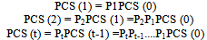 | (1) |
Where Pt is transition probability matrix at time t and PCS(t)is the condition vector at the (t) period. PCS leads to the rail condition quality such as rail wear index or any appropriate scale in the quantitative analysis. All the elements of matrix Pt are transition probabilities. So, here all the elements are between zero and one and the sum of the elements of each row equals one.[3]Semi - Markov model was made using the available data and the experience of professional experts with regard to the permanent way. The main advantage of this type of model is its application of mental sources which reduced the need for collecting field data. Despite Markov model, these models can predict the future condition from the past condition via the transition probability matrix[11].
3. Deterioration Model of Rail
Infrastructure deterioration models are mathematical relationships between a dependent variable, namely deterioration or change in condition, and a set of casual variables, including design attributes, traffic loading, environmental factors, age and maintenance history. The main challenge in developing accurate deterioration models for infrastructure facilities is that the condition is often measured on a discrete scale. However, facility deterioration itself is a continuous process. For example, in reinforced concrete bridge decks, reinforcing steel bar corrosion is gradual and slow or rail wear is done gradually and over a period. Furthermore, in the initial stages, the deterioration processes do not occur at either microscopic scale or subsurface level; thus it is not observed directly whereas indicators of performance are being observed. It is therefore necessary in developing stochastic discrete state deterioration models to correctly account for both underlying unobserved continuous state deterioration process and observed discrete state deterioration indicators[7].To make it more clear and not lose generalization at the same time, the model was developed for the simple bi-variate case where the facility can be in one of only two possible states, namely 1 and 0, with the latter state reflecting a poorer condition. Once a facility underwent a change in state from 1 to 0, then no further changes were possible because the condition could not been improve without a rehabilitation activity. In this research, it was assumed that the track was without maintenance. Consequently, only the first part of the sequence ending in the first time in which a state of 0 was recorded contained meaningful information. The time variable t was set to zero at the time of the most recent rehabilitation or at the time of structure construction. In other words, at t=0, state 1 was recorded. The value of the threshold deterioration k reflected the boundary defining the condition states of zero and one. The time at which the facilities’ deterioration level reached k represented the duration of state 1 and was denoted by t=T.Typically, discrete-time, state-based deterioration models are characterized by transition probabilities for the points at time separated by a constant period Δ, which is usually set at one or two years, the commonly employed inspection periods.The probability of the transition out of state 1 at time t, therefore, is the probability of observing the facility which has already undergone a drop in state (i.e., change in state from 1 to 0) at time t + Δ conditional on an observed facility state of 1 at time t. This conditional probability is denoted by R (t, Δ) and is given as follows: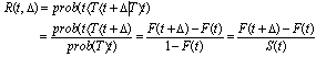 | (2) |
where F (t) = cumulative distribution function of the duration random variable T and S(t)=1-F(t) which is known as the survival function in the stochastic duration modelling literature. Hence, if F(t) is known, R(t, Δ) can be computed for any value of t and Δ. In other words, given a time-based model characterizing the probability density function of the duration T, the transition probabilities of the corresponding discrete-time, state-based model can be readily determined from R(t, Δ).
3.1. Hazard Rate Function
The probability of the transition out of state 1, R(t, Δ), clearly depends on the period Δ. The larger the value of Δ, the higher the probability and vice versa. Therefore, it is convenient to construct a measure that reflects the average rate at which the transition out of a state occurs through dividing this probability by Δ. This measure is represented with .If the facility is monitored almost continuously (i.e., successive observations are taken at very short intervals), then the conditional probability of Eq. 2 divided by Δ is reduced in the following way:
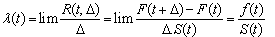 | (3) |
where f (t) =probability density function (PDF) of T; in other words, based on Eqs. (2) and (3), it is the probability of a transition out of state 1 at time t over an infinite small period Δ = dt is . The function
  is known as the hazard rate function in the stochastic duration modelling literature and reflects the instantaneous rate (or risk) at which a facility transits out of its current state to the lower state after time t.
3.2. Duration Model Specification
The functional form of the hazard rate function,  , allows for a convenient interpretation of the nature of the phenomenon being modelled[2]. A constant hazard rate function implies a process in which the conditional probability of the transition out of the state -given by Eq (2) - does not vary over time. This implies that no matter how long time is spent in a state, the probability of the transition out of that state remains constant; hence, it is independent from time. This reflects a process lacking memory and it can be shown that the associated distribution of the duration T follows the exponential PDF. Such a characteristic is referred to as duration independence. A hazard rate function that is monotonically decreasing over time implies that the probability of the transition out of the state decreases with the increase of the time spent in that state. Conversely, a hazard rate function that is monotonically increasing over time implies that the probability of the transition out of the state increases with the increase of the time spent in that state. These characteristics are referred to as negative and positive duration dependence, respectively (See[1] for more details on all three characteristics).As pointed out earlier in this section, once the PDF, f (t), of the duration T is known, the transition probabilities of the corresponding discrete-time, state-based models can be determined. Therefore, the only remaining thing for completing the development of the methodology is the f (t) specification and estimation. Given the intuitive interpretation of the hazard rate function,
  , and its straightforward relationship with the probability density and survival functions given by Eq. (3), it is both convenient and appealing to specify the hazard rate function directly. Once this function is estimated, the PDF of duration can be determined; consequently, transition probabilities can be readily computed. Although material aging and fatigue imply that infrastructure deterioration is in general expected to follow a monotonically increasing hazard rate function (reflecting positive duration dependence), in estimating such a model it is desirable to adopt a single functional form that can cover the spectrum of negative duration dependence, duration independence and positive duration dependence. Such a functional form corresponds to the duration T following the Weibull PDF. The hazard rate function associated with the Weibull PDF is given in the following way:
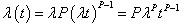 | (4) |
where P and  are the parameters to be estimated.Depending on the value that p takes, the process falls in one of the three duration dependence categories. If 0<p<1, then
  is monotonically decreasing, which reflects negative duration dependence. If p=1, then
  takes the constant value of
  and reflects duration independence, or lack of memory, where the Weibull PDF reduces to the exponential PDF. And, if p>1, then
  is monotonically increasing, which reflects positive duration dependence.It is useful to point out that this explicit treatment of state duration in modelling deterioration reflects a special case of the semi-Markov process. Such a process does not possess the Markovian property due to the presence of duration dependence unless the Weibull PDF takes the form of the exponential PDF. In this special case, the semi-Markov process reduces to a continuous-time Markov chain, where duration independence holds.As already discussed, infrastructure deterioration depends on a set of causal or explanatory variables. Clearly, the Weibull hazard rate function of Eq. (4) does not reflect the effect of such variables. Although this is a serious limitation of this model, its extension to include these variables can be achieved simply by replacing the constant parameter
  with a function dependent on the relevant variables. To ensure that this function is strictly positive, the following exponential specification is adopted:
 | (5) |
where X is the column vector of casual variables (which includes the value one to capture the constant term). In the rail wear model, as the most important casual variable effective on the rail wear is the passing traffic, X only includes one variable which is the passing traffic. So, the X vector is turned into a number and  is the row vector of parameters to be estimated. In wear model, as the X vector is a number, the
  vector is a number, too, which is resulted from drawing exponential diagram of the rail wear breakout index to the passing traffic. Combination of Eqs. (4) and (5) results in the following variable-dependent hazard rate function:
 | (6) |
Under this more general specification, therefore, the duration is now a function of the values of p and X. Note, however, that the nature of duration dependence is still strictly dependent only on p.
3.3. Determining Transition Probability
As discussed before, once the duration model is estimated, the transition probabilities of the corresponding discrete-time, state-based model can be computed. In effect, this amounts to determining the transition probabilities of a discrete-time, state-based process from an estimated semi-Markov process where time is continuous. In the bi-variate case, the probability of the transition out of state 1, which is given by  in Eq. (2), is simply the probability of the transition from state 1 to state 0. Consequently, the transition probability from one state to next state is
  . Under the specification of Eq. (6), where the Weibull PDF and the presence of casual variables are assumed, the probability of remaining in the same state, denoted by P1,1 , is given as follows:
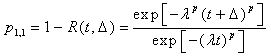 | (7) |
And, the probability of the transition from state 1 to state 0, denoted by P1,0 , is given in the following manner: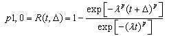 | (8) |
In Eqs. (7) and (8),  is given by Eq. (8). Thus, given an estimated Weibull hazard rate function of Eq. (6), the transition probabilities for the bi-variates case can be computed based on Eqs. (7) and (8) for any point at time t and any period
 .For the multivariate case, the three-state scenario is considered. A duration model for each state is developed exactly similar to the way discussed under the bi-variate case. In this discussion, the three states are denoted by 2, 1 and 0 whereby the additional state 2 is introduced reflecting the situation in which state 2 is the best condition state and 0 is the poorest. In this scenario the remaining elements of transition probability matrix are as follows:
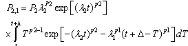 | (9) |
 | (10) |
 | (11) |
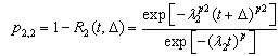
where Ri(t, Δ) =probability of the transition out of state i;  =given by Eq. (5)for state i and Pi=parameter p of Eq. (6) for state i.As in the bi-variate case, the transition probabilities for three state multivariate cases can be computed based on Eqs. (9), (10) and (11) for any point at time t and any period Δ. The extension of the above derivation to the case of more than three states follows a similar treatment.
4. Case Study of Lorestan Railway
To investigate the efficiency of the proposed model, it was tested on one of the lines in Iranian railway network. To do this, Lorestan district was selected due to the problematic rail condition and the presence of numerous curves. The passing traffic from this district was mostly of freight type and it had U33 rail. One of the most prominent features of this district was having a lot of curves with small radius causing more rail wear[13].To make the theory simpler and since the most influential casual variable on rail wear is the passing traffic, it was applied as the only variable in this paper. Besides, to measure rail wear in this district, the data of Line measuring machine, EM120, were applied which measured the rail profile by none contact system per m. Here, the data of three periods with the interval of 6 months Δ=0.5 existed. The first period was on February 4, 2007, the second period was 6 months later and, respectively, the third period was about 1 year later.As the highest amount of wear occurs in the curves, namely, curves with small radius, in this research 2 km of this district located at the curve with 250 m radius was selected as the case study. The highest amount of the wear in the curves was the lateral type of the wear. Besides, in the curves with low passing speed (regarding the freight traffic), the wear occurs on the interior rail; so this paper focused on the lateral wear of the interior rail in each curve. Also, according to the ballasted tracks superelevation technical and general features in Islamic Republic Railway of Iran, the maximum allowable lateral wear for a line with the speed of 60 km/h (D class track) and with U33 rail is 15 mm.The passing traffic in this district was used as model development in 7 years (every year is meaningful from March 21 to the next March 20), from March 21, 2001 with the growth rate of 6% to March 20, 2008, as shown in table 1.[6].| Table 1. The annual passing traffic in Lorestan |
| | 7 | 6 | 5 | 4 | 3 | 2 | 1 | Year | | 3593 | 3389 | 3198 | 3018 | 2860 | 2680 | 2542 | Annual passing freight (1000 ton) |
|
|
To solve the model, the passing traffic from the studied district in each period was required starting from one starting point. So, March 21, 2006 was considered as the traffic basis and the passing traffic was gained from it in each period.After searching the freight and passenger performance bill of lading in railway, it was defined that most part of the passing traffic in Lorestan was of freight traffic and also, due to the volume of the passing traffic near the district capacity, the traffic change rate was fixed every month; this value was 1 in this paper. Then, according to Table (1) and the monthly traffic change rate, the passing traffic was computed in each period.
4.1. The Index Applied in Model Solution and Lines Classification
The condition index is a number computed from an equation and is applied to express the track condition and the level of line servicing. If the condition index is measured in a definite exploitation period, the empirical deterioration function of each index is determined via the condition index diagram against passing Tonnage. This function is of great importance in maintenance management of tracks.The index applied for showing rail condition which was used in this paper can define the amount of rail service. The index is denoted by γ and is defined by the relationship of two areas. If a diagram of wear amount (vertical axial on mm) to kilometre (horizontal axial on m) is drawn, the area under the diagram is displayed by SW. Then, the following equation obviously expresses the definition of this index: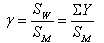 | (12) |
where Sw=the area under the wear amount diagram to the distance. Since the EM120 machine measures the wear data per m, so the wear amount (Y) exists per 1m. Then, the area under the diagram is the sum of wear in 50 points in 50 m parts. SM= the area of allowable wear =lateral allowable wear (15 mm) part length (50m)Two kilometres of the selected area in Lorestan consisted of 10 parts of 200m, all of which belonged to the curves with 250 m radius (some parts are next to each other in one curve and others are in different curves). Then, each part itself was divided to four parts with 50 m longitude. Applying the following definition for the index, first, the index in each 50m part was measured for every period of machine scan; it was gained from the average between 4 parts, the rail wear defect index for each 200m part in each measurement period. Thus, for every 200m part, 3 indexes of 3 measurement periods were available.To determine the lines’ quality, the classification of the lines was done by γ index. This classification was done as shown in Table (2):| Table 2. The classification of the lines on the basis of γindex |
| | 0.75γ> | 0.75 >γ>0.25 | 0.25 >γ> 0 | The scope of γ index | | weak | Average | good | Quality title | | 0 | 1 | 2 | Rank |
|
|
Besides, if the average wear amount (here, 50 points) exceeds the allowable wear boundary (15 mm), that part is in poor condition. In this ranking, rank 2 is the best state and 0 is the worst one.
4.2. Determining Hazard Rate Function λ (t)
To achieve , the exponential diagram should be drawn between γ index and passing traffic. The resulting cure equation was the same as
  equation with traffic (x). According to 10 parts with 200 m long, 10 equations were gained for λ on traffic. On the other hand, for a three-case scenario, as the case study of this research (3 stages of good, average and poor with 3 ranks of 0,1 and 2), λi (λ for state i in which i= 0,1 ,2) is required. As it was not possible to go out of stage 0 or poor state and there was not any worse state than that, so the surviving probability in this state was 1 after one period.
  Consequently, just λ1 and λ2 should be found. Among 10 equations for λ, it was observed that 5 cases were about out of state 2 and 5 cases were about out of stage 1. On the other hand, 5 equations for λ1 and five equations for λ2 were obtained. Out of 5 equations, the one which was fitted with high accuracy and its R2 was closer to 1 should be selected. Thus, the selected λ1 and λ2 that were, respectively, related to the ninth and fifth parts were gained as shown below:
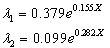 | (13) |
There is another parameter as p in hazard rate function. As said before, since the wear rate change over time is not very tangible, here Pi =1 showed the duration time independence state or memory loss and got weibull PDF of exponential PDF form. By obtaining λi, Pi, λ (t) was easily achieved and applied for transition probability matrix in each period. What follows is about the computation of every transition matrix element in each period. Then, rail wear condition is predicted in a 6-month period.
4.3. Determining Transition Probability Matrix
In the Excel software, the elements were found one by one after preparing one Spirit sheet and giving some inputs such as x (passing traffic), t (time) and Δ (duration of time). Transition probability matrix p for the first 6 month was as follows: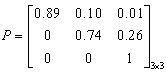 | (14) |
If, at the analysis staring time (t=0), rail was in good condition, rank 2, it can be predicted by this matrix that, according to Eq.(15), the rail will remain in a good condition with the probability of 89%, it will change to the average stage by 10% and to the poor state by 1% during the following 6 months. Once the highest probability was the starting point, it could be predicted that rail wear was in good condition after 6 months.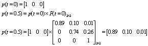 | (15) |
P (t) 3*3 is the transition probability matrix in each period.In the next stage, transition probability matrix p was achieved for the second 6 months as follows: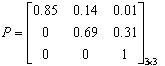 | (16) |
It should be considered that condition vector at t was the starting vector for the next chain, which was different from a transition matrix. Thus, if t ( t=0.5 ), the resulting condition of the first 6 months was considered as the preliminary condition for the second 6 months; in this case, at the beginning of the second 6 months, rail was in a good condition (rank 2) through this matrix. If it had the highest probability, it can be predicted that, after the second 6 months or one year after the analysis, the rail wear remained in a good condition.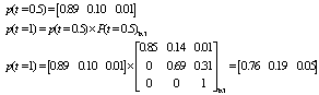 | (17) |
Thus, by the passing traffic and required time, the rail wear condition was predicted with 6 months accuracy.
4.4. Estimating Rail Life on The Basis of Wear
If the mentioned trend in the section4-3 is followed in the next periods, a good approximation of the rail life can be found in the curve with 250m radius. It should be considered that two parameters, time and passing traffic, should be defined. The value of ranking traffic in each period was gained by the 6% growth rate. Time parameter (t) in each period was gained in each period by adding 6 months or half a year to the previous period. To get the rail life, this cycle was continued to the extent that the rail was in the poor condition, considering the highest probability.In the final stage, transition probability matrix P for the sixth (six months) and the condition vector at the end of the sixth period was as follows: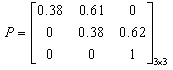 | (18) |
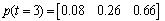 | (19) |
According to Eq..(19), in the investigated zone in the Lorestan district and in the rails with curves of 250 m radius, rail was in a poor condition, considering the analysis starting time after about 6 periods or 3 years, which means that, in February 2010, the rails on the studied zone with 250 m radius should be changed.
5. Conclusions
Applying the proposed model, rail wear condition was achieved with any passing traffic and at any time. In the case study, this process was done for the rail located on the curve with 250 m radius at the period of 6 months. Indeed, by knowing the passing traffic and required time, the rail wear condition was predicted with the accuracy of 6 months. Moreover, using this method, rail life can be predicted and the time for rail replacement can be estimated. To achieve the rail life, the calculation cycle should be repeated to the extent that rail is in the poor state, considering the highest probability. By solving the case using the above method, in the studied zone in the Lorestan district and the rails located on the curves with 250 m radius, , the rail should be in poor state and should be replaced, considering that the analysis started after 6 periods or 3 years. Thus, rail condition can be predicted in future years for other lines of the country and their wear limit can be estimated. In addition, rail life can be estimated and the exact time of its displacement can be determined.It is worth mentioning that, due to 3 periods of rail wear information in the country’s tracks in this research, hazard rate function was just fitted by 3 points. In the case of using the information of more periods, accurate results can be achieved. Besides, the proposed model was applied for predicting other track components and right of other structures.
References
| [1] | Greene, W., Econometric analysis, Macmillan, New York.1997 |
| [2] | Hakhamaneshi, Rambod.: A model for maintenance management of Railway Lines by Markov chain and dynamic planning, case study: Iran Railway, MSc. thesis of Civil Engineering school, Sharif Technical university,2005 |
| [3] | Jobbehdar M.P., Probability theory and applications, Tehran University publication, 2002 |
| [4] | Khaled A. Abaza, P.E.: Iterative Linear Approach for Nonlinear Non homogenous Stochastic Pavement Management Models, Journal of transportation engineering © ASCE , 2006 |
| [5] | Kumar. S.: A Study of the Rail Degradation Process to Predict Rail Breaks, Licentiate thesis،Luleå University of Technology Division of Operation and Maintenance Engineering،2006 |
| [6] | Metra consulting engineers company.: preliminary studies of south district problem solving (region recognition and the existing district traffic), Road and Transportation ministry, transportation infrastructures construction, 2007 |
| [7] | Mishalani R. G. ، Madanat. S. M.: Computation of Infrastructure Transition Probabilities Using Stochastic Duration Models ،Journal of infrastructure systems ,2002 |
| [8] | Mohammadian, Masumeh: Investigation of the stress distribution on the wear rail, B.S thesis of Railway Engineering school, Iran university of science and Technology, 2007 |
| [9] | Ortiz-García J., Costello B., Snaith S., Derivation of transition probability matrices for pavement deterioration modeling, Journal of transportation engineering ,ASCE , 2006 |
| [10] | Shahriari, Sh.: Developing deterioration probabilistic model for rail wear, MSC thesis, school of Railway Engineering, Iran university of science and Technology, 2009 |
| [11] | Smith. R. E.: Infrastructure management System: Course Notes،Texas A&M University،1996 |
| [12] | Technical and general specification of Ballasted Railway, Report No 301, Management and Planning organization of Iran, 2002. |
| [13] | Zakeri J. A. And Rezazadeh M.: railway Track Maintenance Methods, Iran university of science and Technology press, 2007. (in Persian) |
 Abstract
 Reference
 Full-Text PDF
 Full-Text HTML