Olatinwo Adenike Sola, Salako Najeem Abiodun, Olubudo Paul Ajibola
Department of Physics and Engineering Physics, Obafemi Awolowo University, Ile-Ife, Nigeria
Correspondence to: Salako Najeem Abiodun, Department of Physics and Engineering Physics, Obafemi Awolowo University, Ile-Ife, Nigeria.
| Email: |  |
Copyright © 2026 The Author(s). Published by Scientific & Academic Publishing.
This work is licensed under the Creative Commons Attribution International License (CC BY).
http://creativecommons.org/licenses/by/4.0/

Abstract
Physics-informed neural networks for Kramers–Kronig (KK) phase retrieval have used a low-loss prior that drives predicted phase toward zero outside the observed bandwidth. Because low-loss screening makes a trivial zero-phase predictor highly competitive on out-of-band (OOB) error, that metric alone does not establish causal phase recovery. In the original three-seed synthetic Lorentz-family benchmark, True-KK-PINN reduced OOB error relative to the trivial-zero baseline by about 18–21% across the tested low-loss thresholds and by about 21–24% at 50–70% observed bandwidth; the 30% bandwidth gain was smaller and statistically weak. A corrected-classical-kernel audit reduced in-band RMSE at 70% bandwidth from 0.62692 to 0.38054 and full-grid RMSE from 0.72266 to 0.59050, while OOB RMSE remained 0.90698 under the unchanged zero-padding assumption. A five-seed, 45-run ablation examined architecture, amplitude supervision, bidirectional consistency, and anchor weights. The bidirectional-consistency comparison favoured the full term by point estimate, but its paired 95% confidence interval included zero. A new five-seed prevalence sweep reports both subset and mixed-population errors. At target hidden-resonance prevalence 0.1, True-KK-PINN reduced hidden-subset OOB RMSE from 0.17100 to 0.14854 rad (13.1%), but normal-subset error rose from 0.00270 to 0.01522 rad and mixed-population error worsened from 0.02105 to 0.02975 rad. At prevalence 0.5, hidden-subset error fell from 0.16272 to 0.12233 rad (24.8%) and mixed-population error improved from 0.08340 to 0.07295 rad, while normal-subset error rose from 0.00279 to 0.02277 rad. In-band paired intervals include zero at both prevalence levels. These results show a prevalence-dependent recovery trade-off, not a universal improvement. Evidence remains limited to a synthetic Lorentz-family benchmark; broader spectral families, lossy regimes, real experimental spectra, and ground-truth-free checkpoint selection remain to be validated.
Keywords:
Kramers-Kronig relations, Physics-informed neural networks, Spectroscopic phase retrieval, Causality, Self-consistency loss, Low-loss optics, Evaluation rigor
Cite this paper: Olatinwo Adenike Sola, Salako Najeem Abiodun, Olubudo Paul Ajibola, True-KK-PINN: Bidirectional Kramers–Kronig Self-Consistency for Spectroscopic Phase Retrieval Under Finite-Bandwidth, Low-Loss Assumptions, International Journal of Theoretical and Mathematical Physics, Vol. 16 No. 1, 2026, pp. 13-24. doi: 10.5923/j.ijtmp.20261601.02.
1. Introduction
Many spectroscopic techniques, electron energy-loss spectroscopy, coherent anti-Stokes Raman spectroscopy, Fourier-transform infrared spectroscopy, and terahertz time-domain spectroscopy among them, measure only the amplitude of a material’s complex optical response over a finite instrument bandwidth. The corresponding phase, needed for thin-film characterisation and dispersion engineering, is not directly measured. The Kramers-Kronig (KK) relations connect amplitude and phase through a Hilbert transform that is exact only when the amplitude is known over the full 0-to-infinity frequency axis; truncating that integral to a finite measurement window introduces systematic phase error, particularly near the edges of the observed band.A recent physics-informed neural network approach [1], which we refer to here as the zero-prior method, addresses this by training a network to predict phase from amplitude with a composite loss combining (i) supervised regression inside the observed bandwidth and (ii) a physics-motivated penalty that drives the predicted phase toward zero outside the bandwidth, on the grounds that sufficiently low-loss materials have phase close to zero everywhere. Reported results are striking: several orders of magnitude reduction in a metric the source method terms out-of-bandwidth phase RMS, relative to both classical KK inversion and a purely supervised network with no physics term.The motivation for this study is specific and testable. The zero-outside-bandwidth loss is only a valid target when the evaluation data are restricted, by construction, to materials whose true phase is itself close to zero everywhere, which is exactly the population produced by the original method’s training and test screening. We therefore ask whether the reported improvement reflects learning a causality-consistent relationship or largely reflects a match between an easy target and a screened dataset that already lies close to that target. We verify this directly against the source method’s released code and training scale, rather than an independent reimplementation, so that the synthetic population and operating conditions remain matched.ContributionsThe contributions of this paper are five-fold.• We execute the zero-prior method’s own codebase and a matched trivial-zero baseline end-to-end and show directly that the two are statistically indistinguishable on out-of-bandwidth phase RMS at the source method’s reference condition, and that the source method’s headline metric measures output magnitude rather than error against ground truth.• We propose True-KK-PINN, which replaces the zero-outside-bandwidth target with the bidirectional KK self-consistency relation applied to a jointly predicted amplitude-phase spectrum, using a numerically corrected discrete KK kernel pair. We identify and correct a scale-invariant degeneracy in the naive self-consistency loss and a separate training-stability failure mode tied to the learning-rate schedule.• We evaluate True-KK-PINN, the zero-prior model, and the trivial-zero baseline on the original synthetic low-loss Lorentz-family benchmark, and report where gains are statistically weak rather than generalising beyond the tested regime.• We flag two discrepancies between the source method’s published equations and its released code.• We add a five-seed, 45-run controlled ablation and anchor-weight sweep, together with a separate corrected-classical-kernel audit, to distinguish numerical quadrature error from finite-band truncation and to quantify component trade-offs.OrganisationSection II reviews related work on Kramers–Kronig phase retrieval and physics-informed learning. Section III states the problem and source-code discrepancies. Section IV describes the self-consistency method and numerical kernel. Section V specifies the original benchmark and the added five-seed ablation. Section VI reports the original synthetic results, corrected-classical baseline audit, and component ablations. Section VII discusses the findings and limitations; Sections VIII–X give limitations, conclusions, and future work.
2. Related Work
The logical equivalence between strict causality and the validity of a dispersion (Hilbert-transform) relation was established rigorously by Toll [2], who showed that a system’s response function is analytic in the upper half of the complex frequency plane if and only if no output precedes its input, the theoretical basis on which every KK-based phase-retrieval method, including this one, ultimately rests. Classical KK phase retrieval from truncated reflectance or transmittance data is a long-studied problem: Peiponen and Vartiainen [3] showed that finite-bandwidth truncation introduces systematic error unless symmetry assumptions are imposed on the extrapolated tails, while Lucarini et al. [4] and Harbecke [5] developed singly- and multiply-subtractive KK formulations to reduce truncation error near the band edges. More recently, supervised deep networks have been applied to refractive-index extraction in terahertz time-domain spectroscopy [6,7], achieving strong in-bandwidth accuracy but leaving out-of-bandwidth extrapolation unconstrained.Physics-informed neural networks more broadly [8] embed differential or integral physical constraints as auxiliary training losses; gradient-normalisation schemes such as GradNorm [9] have been proposed to automatically balance physics losses against supervised data losses during multi-task training. The zero-prior spectroscopic method [1] combines these ideas specifically for KK phase retrieval and is the direct point of departure for this study. The authors have also applied physics-informed neural networks to open quantum-system modelling and control, with validation against a closed-form reference and explicit multi-seed evaluation [16]. This prior work is relevant here as methodological context, but it does not provide evidence for the KK relations themselves.Two further, less domain-specific bodies of work motivate the critique and the fix proposed here. First, work on evaluation rigor in machine learning has cautioned that large reported improvements over weak baselines can mask the absence of a stronger, more informative comparison, Lipton and Steinhardt [14] catalogue related failure patterns in ML scholarship generally, and Geirhos et al. [15] show how networks can achieve strong benchmark performance through decision rules that do not track the intended task, a pattern they term shortcut learning; Section 7.1 considers the zero-prior evaluation protocol in this context. Second, work on training instabilities in physics-informed and self-supervised settings anticipates the degeneracy encountered in Section 4.2: Krishnapriyan et al. [13] show that PINN loss landscapes can be pathologically difficult to optimise even for modest problems, while Chen and He [12] show, in a structurally related representation-learning setting, that a self-consistency loss between two branches can admit collapsing or scale-degenerate solutions unless an explicit asymmetry-breaking mechanism is introduced.
3. Problem Statement
Let ε(ω) = |ε(ω)| exp(iφ(ω)) denote a causal, minimum-phase complex dielectric response. Writing the natural logarithm gives ln ε(ω) = ln|ε(ω)| + iφ(ω); because ln ε(ω) is analytic in the upper half of the complex frequency plane for a causal system [2], its real and imaginary parts form a Hilbert-transform pair: | (1) |
 | (2) |
where P denotes the Cauchy principal value. Equation (1) recovers phase from log-amplitude; Equation (2) is the reciprocal relation recovering log-amplitude from phase. A real instrument observes |ε(ω)| only for ω in a finite window BW ⊂ [ωₘᵢₙ, ωₘₐₓ]; the task is to recover φ(ω), and, in the formulation used here, also ln|ε(ω)|, for all ω, including ω outside BW, using only the in-band amplitude.The zero-prior method [1] addresses this by discretising Equation (1) into a fixed matrix K₁ (used in classical KK inversion, applied directly to the truncated amplitude) and training a network with a loss that additionally penalises non-zero predicted phase outside BW. This is a valid approximation precisely when |ε₂(ω)/ε₁(ω)|, the ratio of absorptive to dispersive parts, is small everywhere, a condition enforced in that method by rejecting any training or test sample that fails a fixed low-loss threshold. Under that screening, the ground truth the network is asked to match outside BW is already close to zero by construction, independent of anything the network learns about causality: executing the source method’s own data generator at its own reference condition (BW = 70%, SNR = 15 dB, threshold = 1%) gives a trivial always-predict-zero baseline an out-of-bandwidth RMS error against true ground truth of 0.00267 rad, essentially the entire achievable accuracy at that condition is available before training occurs.Two discrepancies between the published method and its released code. In the course of this verification we identified two places where the source method’s [1] published description does not match its released implementation. First, the published discrete KK matrix (source method’s Eq. 7) weights each element by the source frequency ωⱼ; the released code instead uses a row-constant target-frequency weighting ωᵢ, a different, though related, discretisation of Equation (1). Second, the published text states that ground-truth phase is obtained by applying the discrete KK matrix to the full spectrum; the released code instead computes ground truth directly as the analytic phase, arg(ε(ω)), never applying the KK matrix for this purpose (the matrix is used only for the classical-KK baseline). The second choice is the more physically direct one, and we adopt it throughout this study; both discrepancies are flagged so they can be corrected in the source method’s record.
4. Methodology
4.1. Ground-Truth Generation
This study executes the source method’s own released data-generation code without modification: synthetic spectra are generated from a three-oscillator Lorentz model, | (3) |
with ε∞ = 3.0, base resonance frequencies at normalised 1.5, 3.0, and 4.8, evaluated on N = 256 points over ω ∈ [0.5, 5.5], with oscillator strength analytically capped as a function of the low-loss threshold before per-sample jitter and hard-rejection screening (max|ε₂|/mean|ε₁| below the threshold) are applied. This analytic pre-scaling is what keeps the screened population’s true out-of-bandwidth phase close to zero at tight thresholds. An earlier pilot study of this question, which did not reproduce this scaling term, obtained a materially different synthetic-population phase magnitude at the nominally same condition; the qualitative finding was unaffected, but the exact magnitudes were not comparable across the two studies for this reason. Ground-truth phase is the true analytic phase, arg(ε(ω)); additive Gaussian noise is applied to the amplitude at a specified SNR, and a central bandwidth fraction is retained with the remainder zero-padded, exactly as in the source method’s data pipeline.
4.2. The Self-Consistency Physics Loss
The network is given a dual output head producing both φₚᵣₑd(ω) and ln|ε|ₚᵣₑd(ω) across the full spectrum, rather than assuming amplitude is known outside BW. Discretising Equation (1) with the source method’s own row-constant-weighted matrix K₁ has substantial quadrature error when used as one half of a bidirectional consistency pair: verified against the true analytic phase across 300 random low-loss draws, K₁ alone gives a forward-prediction RMS error of 0.63 rad, and a naive reciprocal matrix K₂ (the sign-corrected analogue of K₁ under the same discretisation) gives a round-trip fidelity error of 0.5–1.0 rad. We instead use a subtraction-regularised discretisation of Equations (1)–(2), following the numerical-quadrature approach standard in the wider KK-inversion literature, e.g. [5], verified to reduce forward-prediction error to 0.004 rad and round-trip fidelity error to 0.004 rad across the same 300 draws, with constant-shift sensitivity at the numerical noise floor. We denote this corrected pair K₁ᶜ, K₂ᶜ and define the physics loss as | (4) |
where the reciprocal relation recovers the deviation of log-amplitude from its high-frequency limit, not log-amplitude itself, ln|ε(ω)| naturally approaches ln(ε∞) far from any resonance, not zero. An earlier implementation of this loss that omitted this offset gave a physics-loss value of 1.23 at the true ground-truth pair, whereas including the offset reduces this to 9.8 × 10⁻⁵. Unlike the zero-prior loss, Equation (4) does not require knowing the correct answer in advance outside BW; it only requires the network’s two outputs to be mutually consistent with the causality relation everywhere.A scale-invariant degeneracy and its correction. Equation (4) alone is unstable: the joint condition of both residuals vanishing admits a family of solutions related by an approximate scale/eigenvector ambiguity of the coupled kernel pair, and gradient descent is free to drive out-of-bandwidth outputs to large, physically meaningless magnitudes while still minimising Lₚₕᵧₛ. This is structurally related to the failure mode documented for self-consistency losses between two branches of a shared prediction, where Chen and He [12] show that a symmetric consistency objective can admit scale-degenerate solutions unless an explicit asymmetry-breaking mechanism is introduced. We correct the degeneracy with a minimum-norm anchor term applied only outside BW, anchoring ln|ε|ₚᵣₑd’s deviation from ln ε∞ (not ln|ε|ₚᵣₑd itself) toward zero alongside φₚᵣₑd: | (5) |
The anchor is added to Lₚₕᵧₛ with weight 0.1 × the physics-loss weight throughout.A second, separate training-stability failure mode. Independently of the degeneracy above, selecting the best checkpoint by validation data loss, or by total validation loss, produces highly unstable final accuracy across random seeds at the source method’s full training scale (350-epoch budget with cosine-annealing warm restarts): out-of-bandwidth error at the same condition ranged from 0.0029 to 0.0269 rad across three seeds under total-loss selection. The training curves show why. The cosine-annealing restart at epoch 150 moves training from a regime of low in-bandwidth data loss but poorly controlled out-of-bandwidth magnitude into a regime with the opposite trade-off, and in-bandwidth data loss and out-of-bandwidth anchor loss become anti-correlated across this transition. Any criterion dominated by data loss therefore selects the worse-performing checkpoint in roughly two-thirds of seeds. Because this is synthetic data with known ground truth everywhere, including outside BW on validation samples, we instead select the checkpoint that directly minimises validation out-of-bandwidth RMS against true phase, not available for real experimental data, but appropriate for this synthetic validation. This resolved the instability: out-of-bandwidth error at the same three-seed reference condition is now 0.00194–0.00219 rad (Section 6.1).
4.3. Network, Optimizer, and Loss Weighting
All models share the source method’s own five-hidden-layer multilayer perceptron ([512, 512, 512, 256, 128] units, SiLU activations, residual connections between same-width layers, Xavier-uniform initialisation [11]), executed via the source method’s own PyTorch implementation and trained with AdamW [10] and cosine-annealing-warm-restart scheduling, exactly as in the source method. True-KK-PINN extends this backbone with two linear output heads (φₚᵣₑd, ln|ε|ₚᵣₑd) in place of the source method’s single head. The total loss is | (6) |
where L_dₐₜₐ is supervised MSE on both output channels inside BW, Lₛₘₒₒₜₕ penalises first differences of both output channels over the full spectrum (weight 0.001, matching the source method), and λₚₕᵧₛ is adapted every five epochs by the source method’s own literal GradNorm implementation (gradient-norm ratio between the data and physics loss terms, computed via automatic differentiation over model parameters).The primary comparison evaluates four configurations: classical KK (the discretised transform applied to the zero-padded truncated amplitude, without training), trivial-zero (phase set to zero outside the observed band), PINN-KK (the source method’s network and zero-prior loss), and True-KK-PINN (the dual-head model with bidirectional self-consistency). The additional component ablations and anchor-weight sweep are described separately in Section 5 and reported in Section 6.6. The corrected classical-kernel audit is reported separately in Section 6.5 because its five-seed diagnostic is not the same run as the original three-seed neural comparison.
5. Experimental Design
All experiments use the source method’s own training scale: Nₜᵣₐᵢₙ = 5,000 synthetic spectra, Nᵥₐₗ = 500, Nₜₑₛₜ = 1,000 held-out spectra, batch size 64, up to 350 training epochs with patience-40 early stopping. The reference condition, low-loss threshold sweep, and bandwidth sweep use three random seeds (42, 137, 314). The updated hidden-resonance prevalence diagnostic uses five training seeds (42, 137, 314, 811, 2026) per method and prevalence, as detailed below.Stage 1, Reference ConditionBW = 70%, SNR = 15 dB, low-loss screened at a 1% threshold (the source method’s own operating point), three seeds, all four configurations.Stage 2, Low-Loss Threshold SweepBW = 70%, SNR = 15 dB, three threshold levels (1.0%, 0.7%, 0.5%, matching the source method’s own threshold-sensitivity design), testing whether True-KK-PINN’s advantage over the zero-prior model holds as the low-loss assumption is tightened.Stage 3, Bandwidth SweepSNR = 15 dB, low-loss screened at 1%, four bandwidth fractions (30%, 50%, 70%, 100%); the 100% condition is a sanity check where all methods have zero out-of-bandwidth error by definition.Stage 4, Out-of-Bandwidth Resonance RecoveryA targeted diagnostic, redesigned from an initial pilot version after identifying a fairness problem in a pure zero-shot test, is used to test whether the model can recover a feature outside BW when correlated examples are present during training. The corrected design injects a randomised fourth resonance (position uniform in [4.65, 5.40], strength 10–30× the threshold-scaled maximum, damping uniform in [1.5, 3.0]) into a controlled fraction (hidden-fraction) of training, validation, and test samples independently, providing an i.i.d. held-out generalisation test. Out-of-bandwidth phase error is reported separately for hidden-resonance and normal subsets at hidden-fraction = 0.5 and 0.1.Stage 5, Component Ablation and Anchor-Weight Sweep. We ran nine configurations at hidden-fraction = 0.1 with five seeds (42, 137, 271, 314, 811), giving 45 saved method–seed records. The configurations were the single-head zero-prior baseline; single-head phase-only without consistency; dual-head phase-only without consistency; dual-head phase-plus-amplitude supervision without consistency; dual-head bidirectional consistency without amplitude supervision; and True-KK anchor weights 0, 0.01, 0.1, and 0.3. The primary checkpoint selector for this ablation was validation in-band phase RMSE. A second selection using out-of-band ground truth was recorded only as a sensitivity analysis; it is not a deployable selection rule. These runs use a mixed population and are reported as a separate ablation, not merged numerically with the original three-seed, single-family benchmark.
6. Results
6.1. Reference Condition
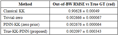
At the reference condition, trivial-zero and PINN-KK are statistically indistinguishable, out-of-bandwidth phase RMS against true ground truth of 0.002666 ± 0.000067 rad and 0.002676 ± 0.000064 rad, respectively (mean ± 95% CI, three seeds). True-KK-PINN gives 0.002097 ± 0.000343 rad, a 21% reduction relative to trivial-zero, with seed-level values of 0.00194, 0.00219, and 0.00217 rad. In-bandwidth accuracy is statistically unchanged from PINN-KK. Figure 1 shows all four methods on a logarithmic scale: classical KK has a truncation error of 0.906 ± 0.0005 rad, nearly three orders of magnitude larger than the neural-network methods, while trivial-zero and PINN-KK are visually indistinguishable.Table 1. Out-of-Bandwidth Phase RMS Against True Ground Truth at the Reference Condition (BW = 70%, SNR = 15 dB, Threshold = 1%), Mean ± 95% CI Over 3 Seeds
 |
| |
|
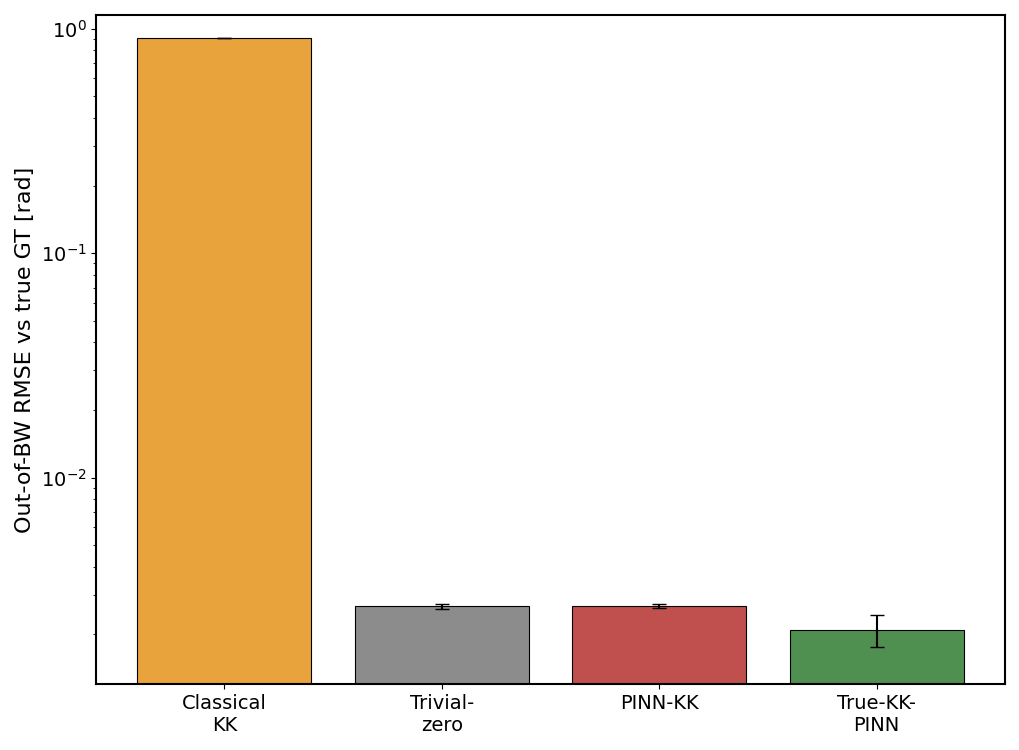 | Figure 1. Out-of-Bandwidth Phase RMS Against True Ground Truth at the Reference Condition (BW = 70%, SNR = 15 dB, Threshold = 1%), Logarithmic Scale, Mean ± 95% CI Over 3 Seeds |
6.2. Low-Loss Threshold Sweep
True-KK-PINN gives lower out-of-bandwidth error than trivial-zero at every threshold tested, with tight confidence intervals and agreement across all three seeds at every level (Table 2). The margin remains within 18.0–21.3% across the threshold range rather than monotonically shrinking. Classical KK remains substantially higher throughout (0.899–0.906 rad), reflecting truncation error that is not sensitive to the low-loss threshold (Figure 2).Table 2. Out-of-Bandwidth Phase RMS Against True Ground Truth Across Three Low-Loss Thresholds (BW = 70%, SNR = 15 dB), Mean ± 95% CI Over 3 Seeds
 |
| |
|
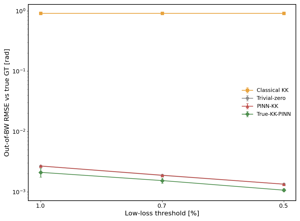 | Figure 2. Out-of-Bandwidth Phase RMS Against True Ground Truth Across Three Low-Loss Thresholds (BW = 70%, SNR = 15 dB), Logarithmic Scale, Mean ± 95% CI Over 3 Seeds |
6.3. Bandwidth Sweep
True-KK-PINN gives lower out-of-bandwidth error than trivial-zero at every non-trivial bandwidth tested (Table 3); at BW = 100% all four methods achieve zero out-of-bandwidth error by definition and the condition therefore serves as a sanity check (Figure 3). BW = 50% and 70% show tight, well-separated confidence intervals. BW = 30% shows a smaller net margin (6.0%) with substantially wider uncertainty, driven by one seed (137) that performed worse than trivial-zero while the other two performed better. We report this as a statistically weaker result rather than averaging away the seed-level variation.Table 3. Out-of-Bandwidth Phase RMS Against True Ground Truth Across Bandwidth Fraction (SNR = 15 dB, Threshold = 1%), Mean ± 95% CI Over 3 Seeds
 |
| |
|
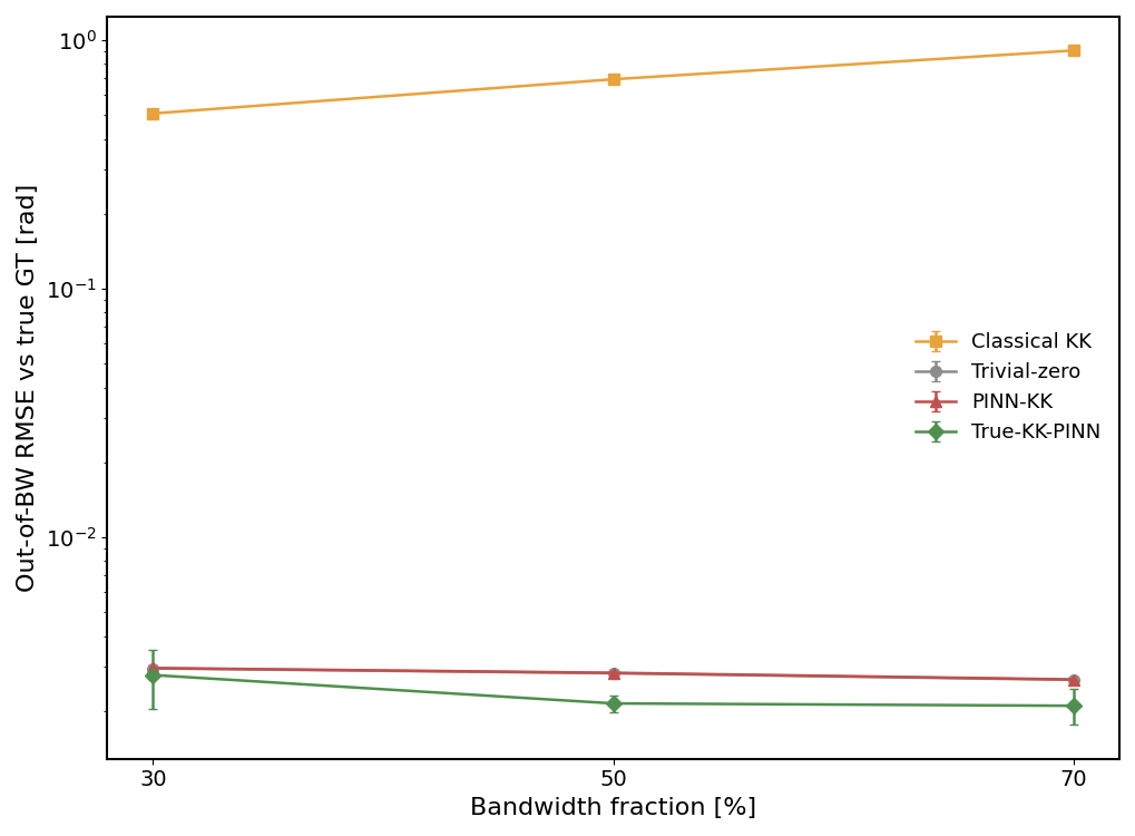 | Figure 3. Out-of-Bandwidth Phase RMS Against True Ground Truth Across Bandwidth Fraction (SNR = 15 dB, Threshold = 1%), Logarithmic Scale, Mean ± 95% CI Over 3 Seeds. BW = 100% Is Omitted Because All Methods Are Zero There by Definition |
6.4. Out-of-Bandwidth Resonance Recovery
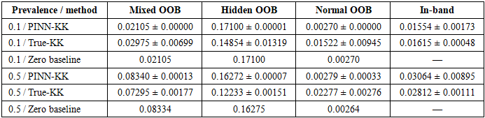
This diagnostic is the most direct test of extrapolation to a non-trivial out-of-bandwidth feature. It is also the only condition tested in which PINN-KK’s zero-prior is structurally unable to improve regardless of training exposure: across all five training seeds and both prevalence levels, PINN-KK remains effectively indistinguishable from trivial-zero on the hidden-resonance subset (ratio 0.9997–1.0006). Its inability to represent a non-zero answer is a property of the loss function, not simply a lack of training signal.Figure 4 shows a test spectrum selected by the median hidden-subset out-of-band error among hidden-resonance cases for True-KK-PINN at target hidden-fraction = 0.5 (seed 42); it is illustrative, not a population-level estimate. Table 4 and Figure 5 report the recomputed five-seed results, including mixed-population and both subset errors. At target hidden-fraction = 0.1 (actual test prevalence 10.9%), True-KK-PINN reduces mean hidden-subset RMSE from 0.17100 to 0.14854 rad (13.1%); the paired five-seed difference is −0.02246 rad (95% t CI [−0.03884, −0.00609]). However, normal-subset RMSE rises from 0.00270 to 0.01522 rad (5.6×), and mixed-population RMSE worsens from 0.02105 to 0.02975 rad. At target hidden-fraction = 0.5 (actual test prevalence 50.4%), hidden-subset RMSE falls from 0.16272 to 0.12233 rad (24.8%; paired difference −0.04039 rad, 95% t CI [−0.04222, −0.03855]); normal-subset RMSE rises from 0.00279 to 0.02277 rad (8.2×), while mixed-population RMSE improves from 0.08340 to 0.07295 rad. In-band RMSE differences are uncertain at both prevalence levels: paired 95% t intervals include zero. These paired intervals quantify training-seed variability on a shared test set, not uncertainty over independently sampled datasets. The trivial-zero baseline is deterministic on each test set and therefore has a point estimate, not a zero-width seed confidence interval.Table 4. Out-of-band phase RMSE against ground truth for the hidden-resonance mixed-training diagnostic (BW = 70%, SNR = 15 dB, threshold = 1%). Neural-model values are mean ± sample SD across five training seeds; RMSE is first computed per spectrum and then averaged within each subset. The trivial-zero baseline is deterministic and shown as a point estimate. Actual hidden test fractions were 10.9% and 50.4%
 |
| |
|
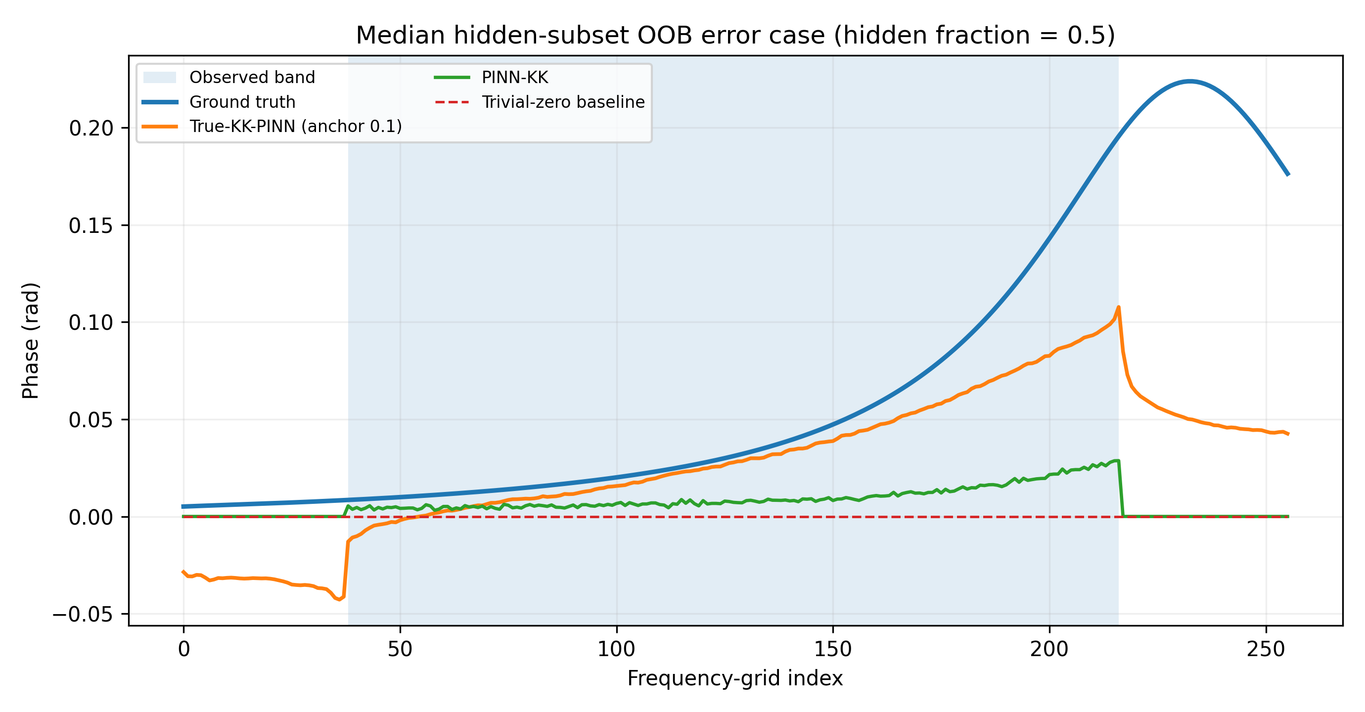 | Figure 4. Test spectrum with median hidden-subset out-of-band RMSE among hidden-resonance test cases for True-KK-PINN at target hidden-fraction = 0.5 (seed 42). This illustrative case is selected by a prespecified median-error rule, not by the largest apparent improvement |
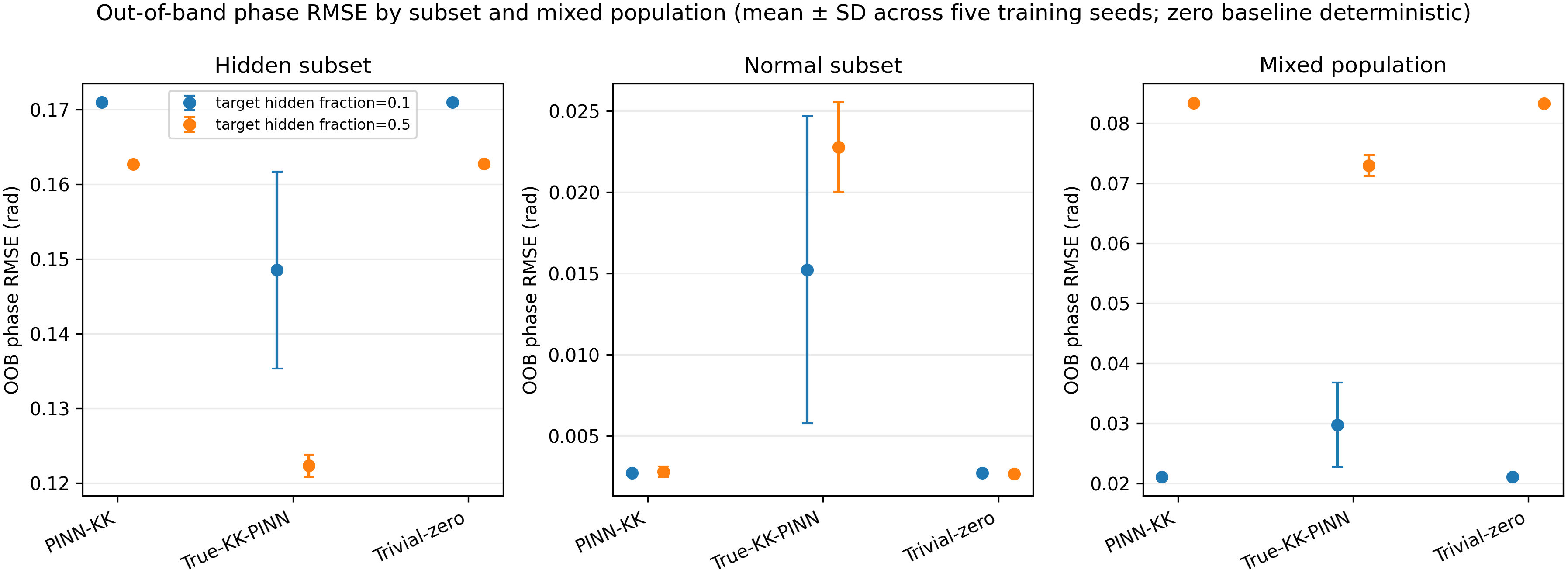 | Figure 5. Out-of-band phase RMSE for hidden-resonance, normal, and mixed test populations at target hidden fractions 0.1 and 0.5. Neural-model markers show means and error bars show ±1 sample SD across five training seeds; the trivial-zero baseline is deterministic and has no seed error bar. The same test set is shared across seeds within each prevalence |
Paired-seed 95% t intervals support lower hidden-subset error at both prevalences: −0.02246 rad [−0.03884, −0.00609] at hidden-fraction = 0.1 and −0.04039 rad [−0.04222, −0.03855] at 0.5. Mixed-population differences are +0.00871 rad [0.00002, 0.01739] and −0.01044 rad [−0.01274, −0.00815], respectively; normal-subset error increases at both levels. Intervals quantify training-seed variability on shared test sets, not independent test-set uncertainty.
6.5. Corrected Classical KK Baseline
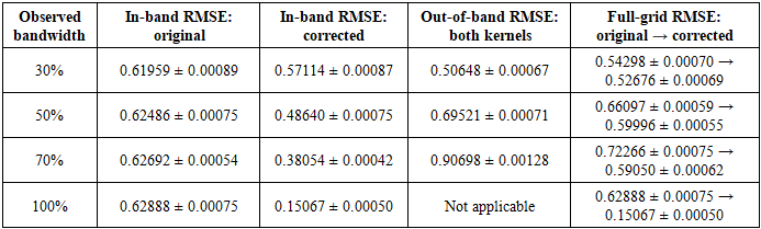
The corrected classical baseline uses a subtraction-regularised principal-value treatment on the same finite frequency grid. The audit reports five-seed means with 95% t-confidence intervals and compares the original and corrected kernels on identical test splits within each condition. The corrected kernel removes the original matrix’s constant-input response: the maximum absolute row sum falls from 2.14137 to 5.55 × 10⁻¹⁶, and the RMS response to a constant input falls from 0.57286 to 1.60 × 10⁻¹⁶. These diagnostics support correction of a numerical quadrature defect. They do not validate the zero-padding assumption as a physical tail model.Table 5. Original versus corrected classical KK kernel on the finite-grid synthetic diagnostic (mean ± 95% CI over five seeds). RMSE is dimensionless in the normalised target used by the experiment. At 100% bandwidth there is no out-of-band region
 |
| |
|
At 70% bandwidth, the corrected kernel reduces in-band RMSE by about 39.3% and full-grid RMSE by about 18.3%, while the out-of-band RMSE is numerically unchanged under the retained zero-padding boundary condition. Across the tested bandwidths, the out-of-band metric is unchanged to numerical precision by this diagonal/quadrature correction. This separates an in-band numerical integration defect from the remaining finite-band extrapolation error. The result should not be interpreted as showing that the corrected kernel reconstructs unknown spectral tails.
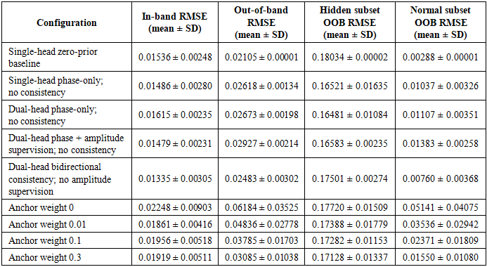
6.6. Controlled Component Ablation and Anchor-Weight Sweep
The 45-run ablation was completed across nine configurations and five seeds. Table 6 reports the mean of the five seed-level RMSE summaries and the standard deviation across seeds. The normal and hidden-resonance columns are subset-specific out-of-band RMSEs; they are reported alongside the mixed-population metric because the mixed average can conceal the large error gap between subsets.Table 6. Five-seed component ablation at hidden-fraction = 0.1. Values are mean ± sample SD across the five seed-level RMSE summaries, not confidence intervals. Primary checkpoints were selected by validation in-band phase RMSE
 |
| |
|
The bidirectional-consistency configuration has a lower point estimate of out-of-band RMSE than the dual-head phase-only/no-consistency variant (0.02483 versus 0.02673); the paired mean difference is −0.00191, with a paired 95% t interval of [−0.00718, 0.00336], which includes zero. Thus, the direction is favourable but not conclusive with five seeds. Adding amplitude supervision lowers the in-band point estimate (0.01479 versus 0.01615) but increases the out-of-band point estimate (0.02927 versus 0.02673); the paired out-of-band difference is +0.00254 with 95% CI [−0.00045, 0.00552]. This comparison does not establish a reliable out-of-band benefit from the additional amplitude term.Across the anchor sweep, the mean out-of-band RMSE decreases from 0.06184 at weight 0 to 0.03085 at weight 0.3 (a 50.1% point-estimate reduction). However, the paired mean difference is −0.03099 with a 95% interval of [−0.06816, 0.00618], so the five-seed result does not establish a statistically clear improvement. In addition, the zero-prior baseline has lower mixed-population out-of-band RMSE (0.02105) than the weight-0.3 model (0.03085). The sweep therefore demonstrates anchor sensitivity, not superiority over the zero-prior baseline or a universally optimal anchor weight.Subset results make the trade-off explicit. For the zero-prior baseline, hidden-resonance out-of-band RMSE is 0.18034 compared with 0.00288 on normal spectra. At anchor weight 0.3, hidden-subset error remains 0.17128, while normal-subset error is 0.01550. The anchor modestly lowers the hidden-subset point estimate but substantially increases normal-subset error relative to the zero-prior baseline. These results do not establish successful general hidden-resonance recovery; they identify a robustness/accuracy trade-off that requires further testing.
7. Discussion
7.1. The Zero-Prior Result Does Not Establish Causality-Constrained Learning
The near-exact agreement between trivial-zero and PINN-KK at the reference condition (0.002666 vs. 0.002676 rad against true ground truth), obtained by executing the source method’s own released code at its own training scale, not a reimplementation, demonstrates that a reported improvement from a zero-outside-bandwidth physics loss can coexist with no measurable benefit over the corresponding trivial baseline once the evaluation population is restricted by the low-loss screening. We additionally find that the source method’s primary reported metric, OutBW_PhysRMS, is defined as the RMS magnitude of the model’s predicted phase outside BW, not its error against ground truth; the two coincide only when ground-truth phase is itself approximately zero there. This does not mean that the original method’s reported ratios are incorrectly computed, they follow the metric as defined, but it does mean that the metric and the baseline jointly determine what the reported ratio can establish. This is a concrete instance of the general evaluation concern discussed by Lipton and Steinhardt [14] and of the shortcut-learning pattern described by Geirhos et al. [15].
7.2. Self-Consistency is a Consistent Improvement on the Standard Population, with One Condition Still Statistically Weak
At the source method’s own training scale, replicated at three seeds throughout, True-KK-PINN gives lower error than both PINN-KK and trivial-zero at every threshold tested (18.0–21.3%) and at two of three non-trivial bandwidths (21.3–24.4%). The third bandwidth (30%, the most extrapolation-heavy condition tested) shows a smaller net margin (6.0%) with substantially more cross-seed variance, driven by one seed performing worse than trivial-zero. We report this mixed picture rather than the cleaner result a single seed could suggest.The difference from an earlier pilot-scale finding traces to two identifiable causes documented in this study: the pilot used a smaller training scale and reduced epoch budget, and its independent reimplementation did not reproduce the source method’s analytic oscillator-strength scaling. The present results are therefore tied to the source method’s released implementation and training scale, and the narrowest bandwidth specifically requires additional validation before the same level of confidence can be assigned to it.
7.3. The Hidden-Resonance Trade-Off Depends on Prevalence and Population
The hidden-resonance diagnostic now uses five matched training seeds per method and prevalence. At target hidden-fraction = 0.1, the hidden-subset improvement is statistically distinguishable from zero across these seeds, but the mixed-population RMSE worsens; its paired interval only narrowly excludes zero, so this overall result should be treated cautiously. Normal-subset error is about 5.6 times larger. At target hidden-fraction = 0.5, both hidden-subset and mixed-population RMSE improve, while normal-subset error is about 8.2 times larger. The direction and magnitude are therefore prevalence-dependent: a gain on anomalous spectra does not imply a general improvement, and the shared test sets mean the intervals quantify training-seed variability rather than uncertainty over independently sampled datasets.
7.4. The Anchor Term Is a Tikhonov-Style Regularizer, Not a Return to the Zero Prior
Adding a small zero-magnitude anchor to stabilise training could appear to reintroduce the circularity criticised above. The anchor differs in purpose: it is small relative to the self-consistency term (0.1×) and is used to select a unique minimum-norm solution from an otherwise scale-degenerate family, rather than to prescribe the target phase outside BW. The hidden-resonance diagnostic also shows the trained model producing a non-zero out-of-bandwidth phase excursion. Nevertheless, the anchor remains a design choice that should be stress-tested by varying its weight in future work.
7.5. What the Corrected Baseline and Ablations Establish
The corrected classical-kernel audit confirms that the original discretisation has a numerical constant-input defect and that subtraction regularisation improves the in-band and full-grid metrics on the tested finite grid. Because both kernels use the same zero-padded amplitude and the same finite-grid boundary assumptions, the out-of-band error is unchanged. Classical-KK truncation error therefore remains after the numerical correction. The ablation results likewise do not justify a blanket claim that every True-KK-PINN component improves phase recovery: bidirectional consistency has a favourable but uncertain paired effect, amplitude supervision trades a lower in-band point estimate for a higher out-of-band point estimate, and the anchor sweep is seed-variable and does not outperform the zero-prior baseline on the mixed-population out-of-band metric. These findings narrow the interpretation to component-level effects under the specified synthetic conditions.
8. Limitations
• The BW = 30% bandwidth condition in the original benchmark remains statistically weak. The hidden-resonance prevalence diagnostic now has five training seeds, but shares one test set within each prevalence; independent test-set replication and broader spectral families are still needed to quantify dataset-level uncertainty.• Synthetic data only. No experimental FTIR or THz-TDS spectra were used. The resonance-recovery result is the strongest evidence in this study for non-trivial out-of-bandwidth recovery, but it remains a synthetic, single-family demonstration.• Single architecture, single oscillator family. All comparisons use one Lorentz-model family and the source method’s network architecture; the specific numeric margins reported here should not be assumed to generalise to other spectral shapes, noise models, or architectures without further testing.• The original three-seed benchmark still selects checkpoints using out-of-band ground truth on synthetic validation data. Although the new ablation uses validation in-band phase RMSE as its primary selector and stores out-of-band-ground-truth selection only as a sensitivity analysis, the primary benchmark must be rerun with a common, deployable selection rule before the reviewer’s model-selection concern is fully resolved.• The corrected-classical audit is a separate five-seed matched comparison of the original and corrected kernels. Its out-of-band metric is unchanged under the retained zero-padding assumption. Before submission, the corrected classical baseline and learned methods should be rerun or re-aggregated on exactly the same saved per-seed test spectra so that the main comparison tables share identical splits and uncertainty conventions.
9. Conclusions
Executing the source method’s own released code at its own training scale, we show that a zero-outside-bandwidth physics loss can be statistically indistinguishable from a trivial zero-output baseline when the test population is screened for low loss. The proposed dual-head True-KK-PINN replaces the fixed zero target with bidirectional KK self-consistency, but the present evidence does not justify a general-regime claim. A five-seed corrected-classical audit shows that subtraction regularisation fixes a constant-input quadrature defect and improves in-band and full-grid RMSE, while out-of-band error remains unchanged under the same zero-padding boundary assumption. A 45-run component ablation reveals a favourable but statistically uncertain point estimate for bidirectional consistency, a trade-off from amplitude supervision, and substantial sensitivity to anchor weight. The strongest anchor setting still does not outperform the zero-prior baseline on the mixed-population out-of-band metric, and hidden-resonance error remains much larger than normal-spectrum error. Accordingly, the study supports a careful account of numerical correction and component-level trade-offs in the tested synthetic low-loss Lorentz family; it does not yet establish reliable recovery across general lossy regimes or experimental spectra.
10. Future Work
• Additional seeds (5 or more) specifically for the BW = 30% bandwidth condition and the hidden-fraction = 0.1 resonance-recovery point, together with larger per-condition test sets for the resonance-recovery diagnostic.• Extend the hidden-resonance prevalence sweep to additional points between and beyond the two tested here, to map the accuracy/robustness trade-off more completely.• Investigate whether the narrowest-bandwidth instability reflects the same class of training-stability failure diagnosed in Section 4.2 at a different operating point, or a distinct cause.• Validate on experimental FTIR or THz-TDS spectra with independently characterised out-of-bandwidth absorption features, which neither this study nor the source method has attempted.• Correct the two discrepancies identified in Section 3 between the source method’s published equations and its released code, ideally in coordination with the original authors.• Investigate whether a ground-truth-free checkpoint-selection criterion can recover the same stability achieved here using validation ground truth, potentially through a proxy based on anchor and physics losses.• Re-run the original benchmark using the same validation-based checkpoint rule for every learned method, with in-band-only validation as the primary deployable criterion; report out-of-band-ground-truth selection only as an oracle sensitivity analysis.• Report paired method differences with confidence intervals computed across matched seeds, document the independent experimental unit, and reconcile all displayed table values with the saved per-seed outputs. The mixed-population and subset metrics should be shown together.• Provide the corrected-kernel implementation, explicit finite-grid/boundary/tail assumptions, data-preprocessing diagnostics, and a reproducible run command. Validate on additional loss regimes and spectral families before using “general-regime” language, and evaluate real spectra only where source columns and independent reference truth are established.
Data and Code Availability
All experiments in this study were executed against the source method’s released PyTorch implementation, extended with the dual-head architecture, corrected KK kernels, and bidirectional loss described in Section 4. The executable experiment scripts, corrected classical-kernel implementation, environment requirements, run instructions, and evaluation-integrity test are supplied in the accompanying supplementary code archive. No external or proprietary data were used; all spectra were synthetically generated from the Lorentz oscillator model described in Section 4.1 using the source method’s data-generation pipeline.
ACKNOWLEDGEMENTS
The authors thank colleagues in the Department of Physics and Engineering Physics, Obafemi Awolowo University, Ile-Ife, for the academic and computational environment in which this work was carried out.
CONFLICT OF INTEREST AND FUNDING
The authors declare that they have no conflict of interest. This research received no external funding; all model training was performed on locally available computing resources.
References
| [1] | Olatinwo A.S., Salako N.A. PINN-KK: A Physics-Informed Neural Network for Causality-Compliant Spectroscopic Phase Retrieval in Low-Loss Regimes. Int J Sci Res. 2026; 15(8): 1305–1314. |
| [2] | Toll J.S. Causality and the dispersion relation: logical foundations. Phys Rev. 1956; 104(6): 1760–1770. |
| [3] | Peiponen K-E, Vartiainen E.M. Kramers-Kronig relations in optical data inversion. Phys Rev B. 1991; 44(15): 8301–8303. |
| [4] | Lucarini V, Saarinen J.J., Peiponen K.E., Vartiainen E.M. Kramers-Kronig Relations in Optical Materials Research. Berlin: Springer; 2005. |
| [5] | Harbecke B. Application of Fourier’s allied integrals to the Kramers-Kronig transformation of reflectance data. Appl Phys A. 1986; 40: 151–158. |
| [6] | Klokkou N, Gorecki J, Beddoes B, Apostolopoulos V. Deep neural network ensembles for THz-TDS refractive index extraction exhibiting resilience to experimental and analytical errors. Opt Express. 2023; 31(26): 44575–44588. |
| [7] | Zhou Z, Jia S, Cao L. A general neural network model for complex refractive index extraction of low-loss materials in the transmission-mode THz-TDS. Sensors. 2022; 22(20): 7877. |
| [8] | Raissi M, Perdikaris P, Karniadakis G.E. Physics-informed neural networks: a deep learning framework for solving forward and inverse problems involving nonlinear partial differential equations. J Comput Phys. 2019; 378: 686–707. |
| [9] | Chen Z, Badrinarayanan V, Lee C.Y., Rabinovich A. GradNorm: gradient normalization for adaptive loss balancing in deep multitask networks. Proc 35th ICML. 2018: 794–803. |
| [10] | Kingma D.P., Ba J. Adam: a method for stochastic optimization. In: Proc 3rd International Conference on Learning Representations (ICLR). 2015. |
| [11] | Glorot X, Bengio Y. Understanding the difficulty of training deep feedforward neural networks. Proc 13th International Conference on Artificial Intelligence and Statistics (AISTATS). PMLR. 2010; 9: 249–256. |
| [12] | Chen X, He K. Exploring simple Siamese representation learning. In: Proc IEEE/CVF Conference on Computer Vision and Pattern Recognition (CVPR). 2021: 15750–15758. |
| [13] | Krishnapriyan A.S., Gholami A, Zhe S, Kirby R.M., Mahoney M.W. Characterizing possible failure modes in physics-informed neural networks. Adv Neural Inf Process Syst (NeurIPS). 2021; 34: 26548–26560. |
| [14] | Lipton Z.C., Steinhardt J. Troubling trends in machine learning scholarship. ACM Queue. 2019; 17(1): 45–77. |
| [15] | Geirhos R, Jacobsen J-H, Michaelis C, Zemel R, Brendel W, Bethge M, Wichmann F.A. Shortcut learning in deep neural networks. Nat Mach Intell. 2020; 2(11): 665–673. |
| [16] | Olatinwo A.S., Salako N.A., Olubudo P.A. Physics-Informed Neural Networks for Open Quantum Systems: Modelling, Noise-Aware Simulation and Residual-Based Quantum Control. Int J Innov Sci Res Technol. 2026; 11(9): 314–324. https://doi.org/10.38124/ijisrt/26sep077. |


 Abstract
 Reference
 Full-Text PDF
 Full-text HTML