1. Introduction

Einstein’s Special Relativity Theory (ESRT) deals with the inertial frames. In real physical cases a frame needs to gain velocity from 0 to v at least once. This requires a theory to connect between non-inertial cases and ESRT. Kinematic Special Relativity (KSR) theory, (non-inertial special relativity), [1] was developed earlier to appropriately describe Special Relativity (SR) in non-inertial conditions. KSR theory was developed by establishing the Space-Time Relation (STR) between two frames in relative motion with simultaneity condition. This was done using the propagation time for the light signal of an event occurring at the synchronization position in the reference frame being simultaneously detected by the traveler and coincident observer in the stationary frame. The simultaneity condition is natural and central to ESRT. The final result of the KSR theory was an integral formula for the STR between two frames.

ESRT uses inertial frames. One of the two frames with relative velocity can be inertial and designated as reference with label F and assumed stationary. The other frame with relative velocity to the previous one either would have gained velocity after being at rest in F or may have the relative velocity from eternity. For the inertial traveling frame F’ case an observer in the stationary frame obtains the STR in the other frame with reference to his own through synchronization. ESRT uses the frames resynchronization after F’ has gained constant velocity. Synchronization with real object or frame F_R that will be moving with F’ is done in KSR when there is no relative velocity between F and F_R. In this case the observed clock times of F_R in F won’t agree with ESRT time in F’ but the incremental time of clocks in F_R and F’ will be identical.

Transition to non-inertial theory can be made with a real frame F_R in F gaining velocity to co-move with an inertial frame F’. Each position of F_R is matched to the position of F’ as it appears in F. Further discussion is presented in Sec. 4 to establish the special relativity theory for real frames or objects.

More research was carried out on the subject of previously published KSR theory and the length contraction concept [2]. In a scenario of a traveler stopping after traveling some duration at constant velocity, the clock in F and one carried by the traveler (t and t_R) didn’t increment equally for some duration. This is a non-physical condition requiring rectification of KSR theory. Discussion on this subject is provided in section 2. A minor modification was needed in KSR theory to prevent a non-physical outcome.

The length contraction in SR theory has been accepted as real [3-7] for a long time (for about a century). But the publication [2] shows the contracted length is really the expanded space of the real frame when it gained velocity. This paper revels ESRT itself contains the length expansion along the direction of velocity for a real frame and the expanded length is observed contracted in the stationary frame. The space expansion as mentioned in the publication [2] over all three dimensions (3D) with clock sped-up, however, generated a problem when light propagation in the direction orthogonal to the direction of velocity was considered. Further research revealed that the space expansion should be only along the direction of the velocity of real frame F_R and co-moving inertial frame F’. More discussion on this topic is presented in section 3 along with the explanation why the reference frame needs to be the stationary (inertial) frame. Length expansion-contraction is further discussed in this section. Explanation of why the space expansion in the direction of velocity alone doesn’t make space anisotropic is given there.

Special Relativity (meaning flat space-time and no effect on STR due to acceleration) theory for real frames or objects is presented in section 4. A traveling real frame cannot be inertial so the special relativity theory for real frames or objects is synonymous to KSR theory and ESRT can be considered a subset of constant velocity interval in KSR. Misconceptions of ESRT have stemmed from the improper use of the reference frame. Switching frames without its implication on STR is the main reason. Section 5 elaborates on the reference frame designation. Resynchronization of clocks in a constant velocity interval in ESTR results in the out-of-sync clocks and simultaneity issue. Section 6 is devoted to this resynchronization issue. Conclusion follows thereafter.

2. More about Kinematic Special Relativity (KSR) Theory

KSR theory is the basis for ESRT applications in the real physical environment. This theory was further scrutinized to make sure that all conceivable velocity trajectories produce real physical STR data. Some earlier part of the previously published KSR theory is repeated here for proper understanding on the subject. The nomenclature used here can be found in the earlier paper [1]. KSR theory is used to relate space-time data of an inertial frame to space-time data of a non-inertial frame with a non-constant velocity trajectory in general. Basically, that entails finding the simultaneity time relation between coincident observers to observe occurrence of an event and its detection at some spatially separated position of those frames. It should be noted that the expanded positions of F_R coincide with F’ along with the positions x’=x_R=0. The time increment applies, so F’ can be used for this discussion. The parameters involved in this case are event time t₀ and t’₀, observation time t and t’, distance between the event and the observation point and u’, information propagation track length L and L’ and event to observer’s point propagation time t_p and t’_p in stationary and traveling frame F and F’, respectively. Computation of t’ involves finding L’, so t’_p = L’/c can be added to t’₀ to obtain t’. In the previous paper t’_p was computed using the incremental time relation between and for a pulse of light traveling from originating at time t₀ and traveling distance L=u. The relation between and is,

(1)

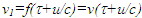where and v are and with The final time relation becomes,

(2)

Eq. 2. Can be represented in the tensor form as,

(3)

in which

In one scenario, t’ was computed for a traveler taking off with constant velocity and stopping at time t_S. According to the previous publication, when was used in Eq. 2, the result showed t’ and t incrementing unequally for some duration after stop time t_S. This non-physical result required rethinking about Eq. 2. The narrative of the first paragraph of this section was scrutinized further. Two different time, t and t₀ are involved in the integration in Eq. 2. ESRT theory uses at the synchronization position. The light signal starts at t₀ at the synchronization position so we need to use at the synchronization position. The incremental light propagation path length and doesn’t occur until the light signal reaches the traveler’s destination at distance u. Therefore, the incremental path length calculation must use the traveler’s velocity at time t+u/c as light signal arrives at his position after traveling distance u. That means we must use instead of in Eq. 1 and 2. Since ESRT connects time relation between observers in relative motion any attempt to formulate a theory based upon the parameters of one observer (data at either x=0 or x’=0) won’t be correct and requirement of confirms that.

Plots involving travel for time t=1 at constant velocity corresponding to and then stop were made with the functionality of and v₁ in Eq. 2 as and in all possible combinations to validate the model of the previous paragraph. Plots in Fig. 1 show the results for the combinations involving and v₁ only. Other combinations involving and v produced non-physical result such as t’ decreasing with increasing t for some duration in certain scenario.

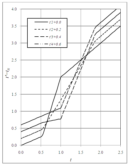Figure 1. Plots showing the time relation between t and t’ for t’1 having γ(τ) and v1(τ+u/c); t’2 having γ(τ+u/c) and v1(τ+u/c); t’3 having γ(τ+u/c) and v1(τ); and t’4 having γ(τ) and v1(τ)

Only for and in Eq. 2 the clocks in F and F’ incremented equally after t=1 as the frames F_R (same as F’ here) stopped. All other plots show non-equal time increment approximately up to time t=2 between clocks of F and F_R even when there is no relative motion between frames. Clock in F_R speeds-up after about t=0.5 due to F_R stopping at t=1. Earlier theories of non-inertial frames do not show any such properties between the time relations and produce unacceptable physical conditions. Plot also shows for F’ stopping at t=1. For the inertial case at t=1 was computed agreeing with ESRT because of the continuing of the relative velocity. Computations for round trip, speed decrease, speed increase and constant acceleration trajectory were performed with the modification as discussed for the KSR theory. The plots t’ vs t relation were somewhat shifted compared to the reported in the earlier publication but adhered to the proper physical behavior.

3. Discussion on the Length Contraction

The current length contraction concept was first advanced by G. Fitzgerald in 1889 [8]. It was hypothesized as the length contraction in the direction of velocity and remained embedded ever since in ESRT. A moving rod not only appears shorter but it is accepted as real effect. It means the rod just doesn’t appear shorter but all physical aspects of the moving rod have to be based upon this shortened length [6-8]. This led to the notion that a moving rod (or axes) will appear rotated if it changed the relative velocity direction. A vast number of notions and publications based on this erroneous shortened length concept exist at present. However, a simple observation can prove that ESRT cannot have real length contraction. In the prevailing SR concept a rod of length L’ in the moving inertial frame F’ is observed contracted as in the stationary “reference” frame F. Length contraction, if real then as the rod stops at time t_S the length L’ will collapse to L in F according this concept. Furthermore, in F’ the rod has out-of sync times so the sections of the rods will continue to move and L’ will collapse to in F’. Such an outcome has no theoretical basis and appears non-physical.

Further reasoning for the absence of length contraction can be provided with the Lorentz Transform (LT) itself which states If we consider an object at x’=X’_ a large value and v=0 then x=X’_ at t’=0. Change, for a small time interval, after t’=0 for F’ gaining sudden velocity v would be according to LT. For a small and LT gives a large spatial change in a small time interval. That is impossible to achieve for a real object. This implies no length expansion or contraction of real frames or objects can be expected in SR.

Synchronization of F and F’ with a constant relative velocity makes F’ a perpetual moving inertial frame. Such perpetual motion is non-physical so F’ cannot be a real frame but it should be designated as a fictitious frame. With this logic a rod of length L1 will correspond to length in F’ as it gains velocity. The length L1’ in F’ will be observed contracted by a factor so the rod itself will be observed having length L1 in F. Thus a rod will be observed of the same length even when it has relative motion. Contrary to the prevailing concept no real length contraction or expansion should be conceptualized in SR.

In the previous publication [2] the real length contraction was shown to be non-physical. The space expansion coupled with the clock sped-up and then length contraction was proposed for more appropriate special relativity theory. Further research showed the space expansion along the velocity direction can be explained within ESRT. Additionally, the space expansion for all directions (3D) stipulated in that publication was found to be in error. 3D expansion produced wrong results for light propagation orthogonal to the velocity direction. 3D expansion and sped-up clock were stipulated to make the space isotropic. Since the inertial space F’ is fictitious it can be anisotropic. However, the out-of-sync time terms in F’ makes it isotropic anyway overcoming the concern of anisotropic space. The length expansion of real objects in F’ coupled with contraction in F make observed dimensions of objects the same regardless of the relative velocity (except some optical illusion with shift of light rays due to velocity). Observed real rod’s length would be same with or without relative velocity due to its virtual space expansion in F’ and then observed contraction (along rod’s length) in F.

The erroneous length contraction concept evolved due to three factors: (i) not recognizing that the moving inertial frame F’ is fictitious while confusing it as a real object or real frame F_R (ii) not properly analyzing the relation between a real and inertial frame if start and stop were included and (iii) casual switching of the reference frame between F and F’ without corresponding STR correction as was pointed out previously [1]. Synchronization of clocks in two frames after one gains relative velocity is obviously going to produce out of synch time. If clocks of both frames were set to zero everywhere when there was no relative velocity then resynchronizing after relative velocity would require varying times in one frame. How can a clocks’ time jump? Such inquiry led to the realization that there is no real length contraction or expansion of length in ESRT.

Representation of F_R as expanded length in co-moving inertial frame F’ can be well illustrated using the reverse process of many prevailing explanation of length contraction such as used with trapping a train in a shorter tunnel. A graphical representation in Fig. 2 illustrates the reasoning. The parameters used for Fig. 2 are and the tunnel length L in F equal to v (t=1). The train and its length is currently accepted real in F’ and is equal to so the train is expected to fit in the tunnel due to length contraction. According to the prevailing narrative [4] the whole train is inside the tunnel in F at t=t’=0 and the exit door position is designated as x=x’=0. But in F’ at t’=0 the caboose position is at x’=-2 and the tunnel’s entrance door at x’=-0.5 value. An observer in F’ sees tunnel too short and doesn’t expect to fit it in the tunnel. For the whole train to be inside the tunnel caboose has to be at the entrance door of the tunnel. This will happen at t’=1.5 at that time t=0 as shown in Fig. 2a satisfying the SR results. The prevailing concept at present to fit a long train in a short tunnel as it trapped is explained by arguing that the train is composed of microscopic sections and each section would enter tunnel at different time in F’ and result in compressed train to fit in the tunnel as shown in Fig. 2b. The trapped compressed train’s length in F is L. In the reverse of trapping the train the compressed train gains velocity at t=0 in F. Fig. 2b depicts the situation. The whole trains gains velocity v at time t=0. The time in F’ at x=x’=0 will be t’=0. The time at x’=-2L in F’ will be t’=1.5 as was the case when the train was stopping. When the caboose is at the entrance of the tunnel at t’=1.5 the exit of the tunnel will be at half the length of the expanded train in F’ with t=0; x=0; t’=1.5 and x’=-2L. The total train length in F’ would be 2L as expanded trapped train length of L.

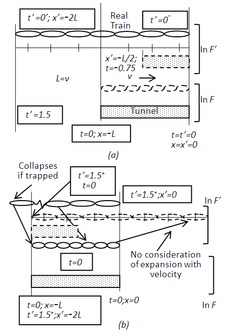Figure 2. Trapping a train in a shorter tunnel scenario according to the prevailing concept in SR (a) as observed in the stationary frame F due to length contraction and (b) showing the compression of the train as it stops but not mention of the expansion in literature as it gains velocity

With the theory presented in this paper the scenario of trapping a train in a shorter tunnel doesn’t arise. The train and the tunnel are observed of the same size in F and F_R. Only in the fictitious frame the train is expanded. Fig. 3 depicts the situation similar to Fig. 2 with the theory presented here. Fig. 4 is the sequence of the real train going through the tunnel of the same length; Fig. 4 (a) is when the train enters the tunnel, Fig. 4 (b) is when it is completely in the tunnel and Fig. 4 (c) is when it leaves the tunnel.

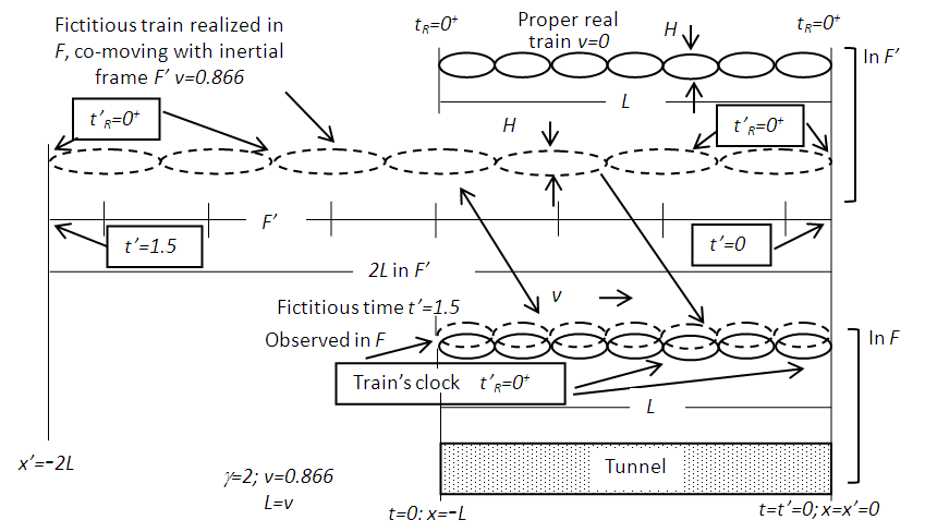Figure 3. Detailed prevailing concept of trapping a train in a shorter tunnel is shown in. The train which is proper length of 2L in F’ is observed physically shorter in F and fits into the tunnel of proper length L when tunnel closes, and gets compressed to the proper length L in F. (b) With the same prevailing concept a shorter proper length L train in F should expand to proper length 2L in F’ when it gains velocity

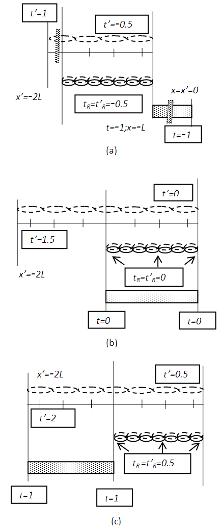Figure 4. Trapping a train in a shorter tunnel scenario according to the prevailing concept in SR (a) as observed in the stationary frame F due to length contraction and (b) showing the compression of the train as it stops but no mention of the expansion as it gains velocity

It is surprising that researchers and experts in the past changed the reference frame from F to F’ and vice versa and concluded that the proper rod length will be observed contracted in the relatively moving frame. It is shown in [1] that changing the reference frame requires length correction and is the correct result and the length contraction of F’ observed in F makes the observed length of a rod same regardless of its relative velocity.

4. Special Relativity for Real Frames

The space expansion stated in [2] is in-line with the above explanation except 3D expansion was in error. Only the space expansion along the velocity direction is correct. In fact it is not the space expansion. It is the representation of a real frame F_R as it gains relative velocity and co-moves with an inertial frame F’ in the reference frame F (usually a stationary frame). This is in contrast to the concept mentioned by Krane [9] as just observing a relatively moving object contracted. The object will be observed same regardless of its relative motion.

For better understanding we introduce proper time, length and co-ordinates t_R, L_R and x_R, respectively for a real frame F_R in one dimensional case. Frames have x=x’=x_R=0 with F_R stationary in F at t=t’=t_R=0. That sets clock times for all x and x_R identical equal to zero. Frame F’ is inertial and is moving with constant velocity v so t’ observed in F will not be proper except at x’=0. Frame F_R gains velocity v at time t=0⁺ and co-moves with F’. Since space and clocks in F_R cannot jump, values x_R=x and t_R=t=0 will persists for t=0⁺. Because the proper length in F’ appears contracted in F a length L_R would exactly match in F’ to the proper length and no sudden change of co-ordinate of F_R in F need to be contemplated. A moving object or frame F_R would appear the same in F regardless of its relative velocity and no anisotropic space arises in the theory. Time increments equally at all positions in F’ so same will happen in F_R and identical time t_R in F_R will be observed at all positions in F. Position x’=0 and x_R=0 will be coincident and the moving observer will have x=vt value in F. These results suggest the Special Relativity theory and Lorentz transformation should be modified for the real frame F_R gaining constant relative velocity in F after the start as:

(4)

Eq. 4 shows the clocks of a real frame F_R with a constant velocity after start in a stationary frame F will be observed identical independent of their position in F_R. The length of a moving object in F_R will appear the same in F regardless of its relative velocity. The inertial frame F’ only serves a procedural tool to relate times in two frames having a constant relative velocity. It is simply imagined in F as a mathematical tool. However, KSR theory requires light propagation path length or incremental time relation as given in Eq. 2 for a non-inertial trajectory of F_R. The simple time relation doesn’t provide the needed data to satisfy the simultaneity condition. The incremental light propagation path length and time relation for a given relative velocity as discussed for the KSR theory needs to be used in non-inertial situation.

5. Reference Frame Selection

For the real frames the symmetric relations of Lorentz transformation doesn’t hold according to Eq. 4. With a constant relative velocity the stationary observers will see a clock’s time in F_R as dilated (running slow) but the observers gaining velocity would see the clock’s time of F as contracted (running fast) according to Eq. 3. In general, in a non-inertial case the time relation between two frames will not be same over the duration of constant velocity as illustrated in Fig. 1.

A question arises how the traveler would observe the stationary frame and obtain STR? For that, only the frame that doesn’t change velocity (like stationary frame) must be designated as the reference frame. This requirement is basic not appreciated in the prevailing understanding of ESRT. Frame F and F_R must maintain the consistent time relation after synchronization without relative velocity. A wave-front generated at the synchronization is observed with the proper time at all places and all durations in F. This is not true in F_R if it changes velocity. This means all computations of STR must be based upon the reference frame F. In that case the traveler with constant velocity must use the same computation as in Eq. 2 making and then follow his trajectory in F. The symmetry of LT that makes STR symmetric also has symmetry for frames F and F’. Switching computation from one frame to other also switches the reference frame. That is OK for the two inertial frames but it is in error for two real frames. Without realization of this fact many paradoxes and misconceptions have occurred with ESRT.

In ESRT both F and F’ are inertial so if we consider F as the stationary (no change of velocity or acceleration over time) real frame then length and time are well defined in F and that is why it is selected as the reference frame. However, with perpetual velocity of F’ or resynchronization after velocity gain the length and time of F’ cannot be compared to the same in F but can be observed only. Therefore, F’ cannot be considered as real frame; but it should be accepted as the virtual frame. Prevailing ESRT use same length data for F’ as was before gaining velocity and clocks are reset in F’. Why the data of F_R need to change as it co-moves with F’ ? Only the positions of F’ and F_R need to correspond properly like map or photo. Clocks in F_R will maintain their value while going from no relative velocity to gaining velocity state. Identical time and position data of real frame F_R before gaining velocity will persist at t=0⁺. The out-of-sync time terms of F’ used in ESRT has no real use in obtaining the STR when the KSR theory is considered. Clocks of both F and F_R are synchronized when there is no relative velocity and the time increment in F_R is same at all positions like in F’ according to the KSR theory and ESRT.

The important point is the synchronization of clocks in F and F_R must be done when there is no relative velocity, the frame that gains velocity is F_R and the stationary frame is F in which clocks have the same time at all positions. Any attempt to find STR using same time at spatially separated positions in a frame makes that frame the reference frame and produces erroneous data if the frame is not stationary (inertial). All STR must be based upon the KSR theory with F as the reference frame. Incidentally, earth is used as the reference frame because it is not expected to gain velocity after synchronization. In that case only the earth can be the reference frame consequently the reciprocity of Lorentz transformation is not for the real world.

6. Discussion on KSR’s Subset ESRT and Misconceptions

A general non-inertial trajectory of a traveler A_R in F_R co-moving with A’ in frame F’ relative to a stationary (inertial) observer A in frame F is considered. In this trajectory one or more intervals may be with constant velocity. In a constant velocity interval ESRT and LT are applicable. Two items; (i) a constant position in a frame and other (ii) equal time at spatially separated positions in a frame are of significance. A large extent frame cannot be expected to gain high velocity making a frame like earth as the stationary (inertial) frame F as the reference frame. Traveler A_R gains high velocity so his real frame F_R cannot have large extent. The co-moving fictitious frame F’ can be of any extent but has no real physical significance for x’ except at x’=0. This means time relations between two frames for some interval with x’=0 has the significance. The short extent of F_R makes the spatial separation in it meaningless so the physical significance of the item (ii) is with equal time t at spatially separated positions in F.

The first item occurs in the case of observing the muon dilated life time. The important aspect in this item is the synchronization before or after has no impact on the theory. That is because the positions and clocks of A_R, A and A’ match; x_R=x=x’=0 and t_R=t=t’=0 as A_R gains velocity.

The item (ii) is the part of misconceptions because it depends upon the clock synchronization process. In ESRT a prevailing concept is “two spatially separated simultaneous events in a frame are not simultaneous in the relatively moving frame [10].” This is true if the synchronization of the clocks in two frames was performed after A_R gained velocity. If the synchronization of clocks was done when F and F_R didn’t have relative velocity then those events will be observed simultaneous in both F and F_R frames. Clarification of this point also shows, in ESRT if clocks time in F’ are set to match with F at synchronization t=t’=0 then non-simultaneous observation and out-of–synch clocks would not arise. Setting of clocks in F’ at the synchronization can be made with some different rule, such as identical to F for ESRT. In that case there will be no out-of sync time but the incremental time will still be related to according to ESRT.

7. Conclusions

Special relativity theory applicable to real frames or objects is presented in this paper. Because two real frames cannot have perpetual constant velocity non-inertial SR, as named KSR theory, is developed here. Minor modifications of the previously published results were required to eliminate non-physical time relation is some scenarios. A detailed discussion of the results of ESRT itself was provided to show length expansion of an object with the gain of velocity but the same expanded length being observed contracted in the stationary frame. This result shows the current concept of the real length contraction in ESRT is in error and objects would appear same with or without relative velocity. Importance of what constitutes the reference frame is highlighted.