Hilmi Ünlü
Fatih Sultan Mehmet Waqf University, Faculty of Engineering, Department of Electrical and Electronics Engineering, Sütlüce, Beyoğlu, İstanbul, Turkey
Correspondence to: Hilmi Ünlü, Fatih Sultan Mehmet Waqf University, Faculty of Engineering, Department of Electrical and Electronics Engineering, Sütlüce, Beyoğlu, İstanbul, Turkey.
| Email: |  |
Copyright © 2023 The Author(s). Published by Scientific & Academic Publishing.
This work is licensed under the Creative Commons Attribution International License (CC BY).
http://creativecommons.org/licenses/by/4.0/

Abstract
We re-examined the four-dimensional spacetime formulation of invariance of electromagnetic fields between two inertial frames under Lorentz transformation, which predicts a pure electric (magnetic) field in one inertial frame is composed the Cartesian components of a pure both electric and magnetic fields in another inertial frame. This contradicts the Lorentz invariance condition which requires that the vector quantities in one inertial frame must have the same form in another inertial frame. In this work, we introduce a three-dimensional quasi-time vector to modify the classical four-dimensional spacetime (3+1) to a new six-dimensional spacetime (3+3) and derive spacetime metric equation and relativistic velocity. We use the classical vector transformation theory to derive expressions for Cartesian components of relativistic velocity and net electromagnetic force vectors. Considering two massive inertial frames form a closed system, we integrated the transformed relativistic velocity with the law of conservation of energy to prove that contrary to the common belief, the electromagnetic field that appears as a purely electric (magnetic) field in one massive inertial frame, it also appears as a pure electric (magnetic) field in another massive inertial frame under Lorentz transformation. As an application of the proposed six-dimensional spacetime theory, we prove Lorentz invariance of Maxwell’s equations with and without charge and current source. We also prove the scalar electromagnetic wave equations with and without charge and current source and the conservation laws of the continuity equations of current and densities of electromagnetic energy and linear and angular momentums between two massive inertial frames under Lorentz transformation.
Keywords:
Six dimensional spacetime, Lorentz transformation, Massive inertial frames, Relativistic velocity transformation, Invariance of electric and magnetic fields, Maxwell equations, Scalar electromagnetic wave equations, Conservation laws for current continuity and electromagnetic energy and momentum
Cite this paper: Hilmi Ünlü, Relativistic Invariance of Electromagnetic Fields and Maxwell’s Equations in Theory of Electrodynamics, International Journal of Theoretical and Mathematical Physics, Vol. 13 No. 2, 2023, pp. 36-56. doi: 10.5923/j.ijtmp.20231302.02.
1. Introduction
Maxwell’s equations and Lorentz force are the foundations of the electromagnetic theory and describe how the charge and current sources with densities  and
and  generate electric and magnetic fields (
 and
and  ), and Lorentz force (
 ) acting on a charge q moving with velocity
  [1]:
[1]:  | (1) |
 | (2) |
 | (3) |
Maxwell’s equations lead to several conservation laws in electrodynamics [1], such as equations of current continuity and laws of conservation of electromagnetic energy and momentum. Historically, Einstein [2] proved the validity of Maxwell’s equations in inertial frames by using Lorentz transformation [3] and proposed two postulates; (i) The laws of physics are invariant in all inertial frames moving with uniform velocities relative to one another. (ii) The speed of light in vacuum is the same in all inertial frames and is independent of the direction of the motion of the emitting body. Einstein combines the rates of change of linear momentum ( ) and energy
  and, after some complicated algebra, finds expressions for the Cartesian components of electric and magnetic fields in inertial frames moving relative to each other along the x-direction [2]
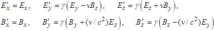 | (4) |
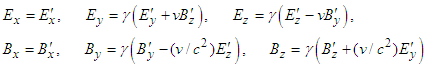 | (5) |
where  is known as Lorentz factor. Here v is the speed of the inertial frames moving relative to each other and c is the speed of light in vacuum. Equations (4) and (5) state that electric and magnetic fields are Lorentz invariant along the direction of motion (x-axis) while there is a change along the perpendicular directions (y, and z-axes). Close inspection shows that although the scalar product of electric and magnetic fields is invariant, their vector product is not invariant between two inertial frames under Lorentz transformation. This has serious impact on the invariance of Maxwell’s equations, electromagnetic wave equations, and conservation laws such as continuity equation of current and electromagnetic energy and momentum between two inertial frames. Therefore, current formulation of the invariance of electromagnetic fields and Maxwell’s equations between two inertial frames under Lorentz transformation remains to be one of the century long unsolved problems [4]-[7]. In this article, our aim is to prove the relativistic invariance of electromagnetic fields and Maxwell’s equations between two inertial frames under Lorentz transformation. The outline of the presentation is as follows. In section 2 we introduce a three-dimensional quasi-time vector to modify the classical four-dimensional spacetime (3+1) to a new six-dimensional spacetime (3+3) and derive spacetime metric equation and relativistic velocity. In section 3 we use the classical vector transformation method to derive Cartesian components of position, relativistic velocity and electromagnetic force vectors in six dimensional spacetime. In section 4 we use the transformed velocity in the law of energy conservation to prove that contrary to common belief, the electric (magnetic) field in so called a massive inertial frame is composed of electric (magnetic) field in another massive inertial frame. In sections 5 and 6 we prove the invariance of Maxwell equations and electromagnetic wave equations between two massive inertial frames.
2. A six-Dimensional Spacetime Frame
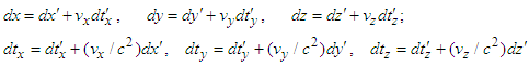
In this section, we introduce time as a three-dimensional quasi-time vector  and
and  , along with three dimensional position vector
  and uniform velocity
  , in three-dimensional space to modify the four-dimensional spacetime (3+1) to define a six-dimensional spacetime (3+3). This idea was first proposed by Mignani and Recami [8] and used by others [9]-[16]. They added two extra time coordinates in the primed and unprimed 4-dimensional inertial frames
 and
and  to interpret the imaginary quantities in the superluminal Lorentz transformations. Time is taken as a vector in the Euclidian 3-dimensional space
  , so that an event can be represented in Euclidian 6-dimensional space
  as
as  . Cartesian components of position vector do not have any physical meaning for tachyons [8], but the magnitude of time vector
  is observable for bradyons [9]. Pappas [13] later on proposed the time vector as
  in Euclidian 3-dimensional time space
  so that an event is represented in a 6-dimensional Euclidian spacetime
  as point
  described by the set of linear equations [13]-[16]
 | (6) |
where  is Lorentz factor, which is anisotropic along the
  and
and  axes in the so called six-dimensional massive inertial frames
  and
and  rather than inertial frames. A laboratory or an observatory in which a free body is observed to retain its motion is considered as examples of massive inertial frames. In this work, we extend our recent work on special relativity [17], [18] to study the relativistic invariance of electromagnetic fields. The theory is based on a six-dimensional spacetime in which two massive inertial frames
  and
and  initially coincide with an absolutely stationary inertial frame
  at time
  . We assume that Einstein’s two postulates are also valid in the 6-dimensional spacetime in which we allow time (space) change in all three Cartesian coordinate axes. We assume that the massive inertial frames
  and
and  move relative to each other with a three-dimensional uniform velocity
  . Time is taken as three-dimensional quasi-vector
  . Here
  ,
,  ,
,  and
and  ,
,  ,
,  in spherical polar coordinates. The magnitude of quasi-time vectors in the massive inertial frames
  and
and  and
and  is measurable and Cartesian components
  and
and  are treated just as mathematical tools in the formulation [9]-[16]. We adopt Einstein’s four-dimensional spacetime formulation of the special theory of relativity [2]. We consider an event of sending a light signal from point
 and second event of the light signal arrival at point
  in the six-dimensional massive inertial frame
  . The coordinates of the events are related to each other by the following relation
 | (7a) |
We can write the following relation for the same two events at points  and
and  taking place in the second six-dimensional massive inertial frame
 | (7b) |
where  according to Einstein’s second postulate. Defining the coordinates of two events as
  and
and  in
in  and
and  and
and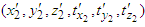 in
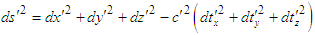
in  , we can write the following six-dimensional spacetime intervals
  | (8a) |
 | (8b) |
as the intervals between the events taking place in the six-dimensional massive inertial frames  and
and  .Just as in the case of four dimensional spacetime theory of special relativity [2], the intervals describing the motion of the simultaneous events in six-dimensional massive inertial frames can be positive (space like separation), negative (time like separation), or zero (null separation). A pair of events with null separation can be connected by a signal at the speed of light. The intervals of two event infinitely close to each other in the massive frames
  and
and  are written as
 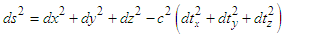 | (9a) |
 | (9b) |
where the differential spacetime along the coordinate axes are defined as [17], [18]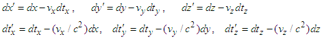 | (10a) |
 | (10b) |
The intervals in Eqs. (9a) and (9b) are related to each other by a metric equation [17], [18]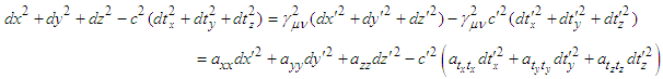 | (11) |
where  are speed dependent coefficients and are given by the following coupled equations
 | (12a) |
 | (12b) |
Setting  transforms covariant equation (11) into the following invariant form
  | (13) |
which states that, just as in the three dimensions, the relativistic quantities (such as velocity and electromagnetic field) should be invariant between two massive inertial frames under Lorentz transformation. Solving the coupled equations (12a) and (12b) for  , one then finds
 | (14) |
which are 6-dimensional analogue of classical Lorentz scaling factor. Square of Lorentz scaling factor  forms a (6x6) orthogonal boost matrix and metric Eq. (11) can be written as
 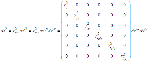 | (15) |
We then write the following matrix equation for line elements in the massive inertial frame 
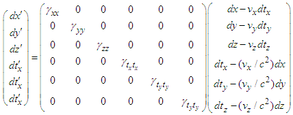 | (16) |
In frame  , one replaces
  with
with  and primed and unprimed subscripts in Eq. (16). One then writes
 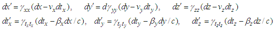 | (17a) |
 | (17b) |
Figure 1 shows the variation of Lorentz scaling factor components  and
and  with azimuthal angle
  for polar angle
  and speed ratio
  . Figure 1 suggests the replacement of classical Lorentz scaling factor
  in four -dimensions with its analogue
  in six-dimensions.
 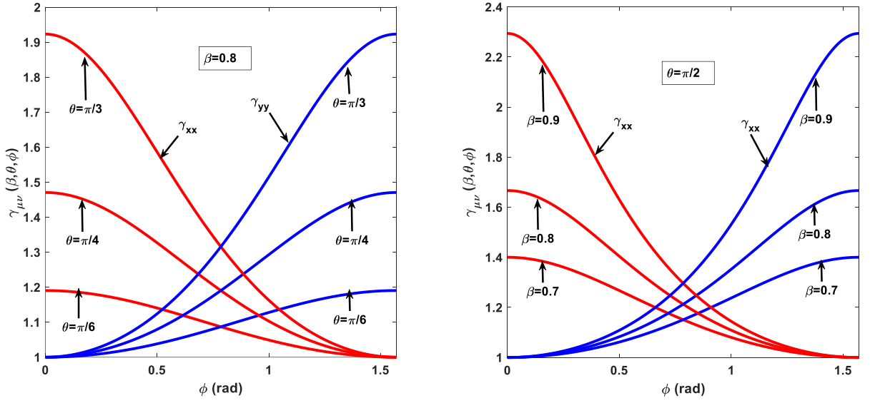 | Figure 1. Angle variation of Lorentz scaling factors  (red line) and (red line) and  (blue line) for (left) (blue line) for (left) 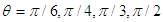 and (right) and (right)  ratio=0.60, 0.70, 0.80 and 0.90 and ratio=0.60, 0.70, 0.80 and 0.90 and  in six-dimensional spherical spacetime coordinates as in six-dimensional spherical spacetime coordinates as  frame moves relative to frame moves relative to  frame frame |
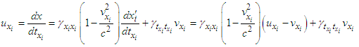
Using Eqs. (17a) and (17b) with  ,
,  and
and  , we can write the following expressions for Cartesian components of the relativistic velocities
  and
and  of an event taking place in massive inertial frame
  and observed in another massive inertial frame
  [17], [18]
 | (18a) |
 | (18b) |
 | (18c) |
When  moves parallel to x axis of
  at the speed of light, Eqs. (18a) - (18c) give
  and
and  (
( and
and  ,
,  and
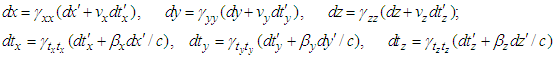
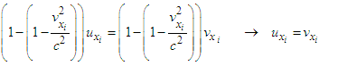
and  ), in agreement with 4-dimensional theory [2]. In order to extend the range of the validity of Eqs. (18a), (18b) and (18c) to any relative speed we combine Eqs. (17a) and (17b) and write x, y and z of
  and
and  in frames
  and
and  , respectively
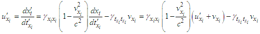 | (19a) |
 | (19b) |
which gives the velocity of an event taking place in frame  and observed in frame
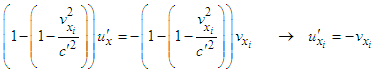 | (20a) |
 | (20b) |
The negative sign means that an event is taking place along + direction in the in frame  and observed in -x direction in frame
  . Equations (20a) and (20b) can explicitly written as
 | (21a) |
 | (21b) |
Figure 2 shows plot of Eqs. (20c) and (20d) for x and y components of  and
and  at speed of light. As the polar angle increases from
  to
to  , the magnitude of components of
  and
and  velocity increase and become unity at
  . The overlapping values of the x and y Cartesian components of
  and
and  suggest an interaction effect between the events. Equations (20c) and (20d) suggest that
  components of
  and
and  components of
  can be determined by using the relative speed of two frames, without requiring one of the unknowns to be known.
 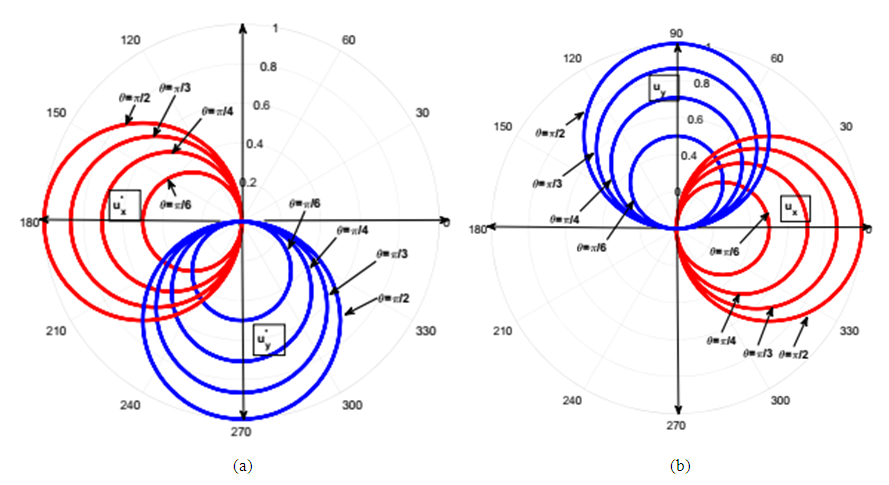 | Figure 2. The plot of x- and y- components of  (Fig. 2a) and (Fig. 2a) and  (Fig. 2b) of an event taking place in massive inertial frame (Fig. 2b) of an event taking place in massive inertial frame  and observed in massive inertial frame and observed in massive inertial frame  as a function of azimuthal angle as a function of azimuthal angle  for polar angle for polar angle 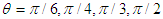 |
3. Relativistic Vector Transformation
In this section, we discuss the classical vector transformation [19] to lay down the groundwork for the study of the invariance of electromagnetic fields between two massive inertial frames. For now, we momentarily set aside the relativity and focus on the transformation of ordinary vectors (i.e., space position, velocity, and force) in three dimensions. The massive inertial frames  and
and  coincide with a rest (an absolutely stationary) inertial frame
  , at
, at  and have common z-axis (
 , in Fig. 3). We define unit vectors
  in the massive inertial frame
  in terms of unit vectors
  in the massive inertial frame
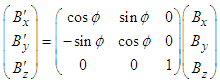
  by using the following linear transformation matrix equation
 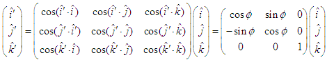 | (22a) |
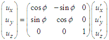
Setting  in Eq. (21a) we can relate
  in frame
  to
to  in frame
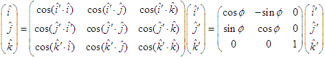 | (22b) |
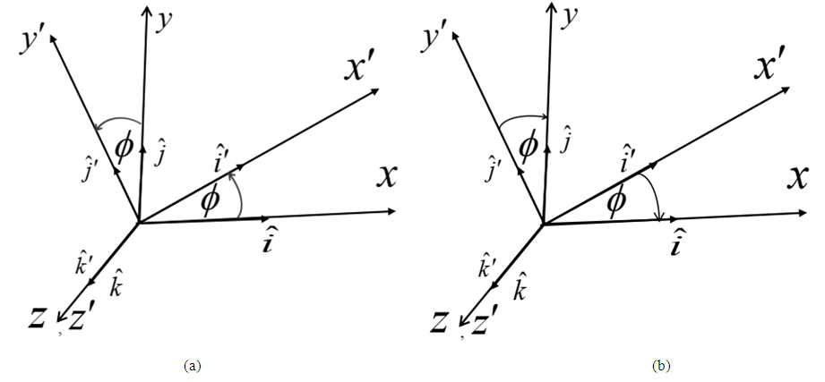 | Figure 3. The schematic diagram of unit vectors in a rotation through azimuthal angle  in counterclockwise of in counterclockwise of  plane into plane into  plane (a) and in clockwise of plane (a) and in clockwise of  into into  plane for plane for  and and  . In both cases . In both cases  or or  axes are kept the same axes are kept the same |
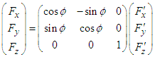
We now consider the transformation of Cartesian components of position, velocity and force vectors. The translation of a position vector does not affect its Cartesian components [19], which transform under rotation according to Eqs. (22a) and (22b). We define three-dimensional stationary position vectors  and
and  in the inertial frames
  and
and  relative to unit vectors
  and
and  , as shown in Fig. 4, by the following equations
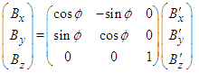
  | (23a) |
 | (23b) |
which can be written in the form of transformation matrix equations for Cartesian components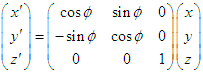 | (24a) |
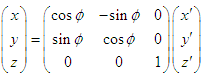 | (24b) |
 | Figure 4. The schematic diagram of  and and  in terms of unit vectors in a rotation through angle in terms of unit vectors in a rotation through angle  in counterclockwise of in counterclockwise of  plane into plane into  plane (a) and in clockwise of plane (a) and in clockwise of  into into  plane for plane for  and and  . In both cases . In both cases  or or  axes are kept the same axes are kept the same |
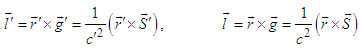
The scalar product of  with itself in
  (or
(or  in
in  ) frame leads to
  , which states that the magnitude of the position vectors
  and
and  Lorentz scalar and have the same length
  from the origin. The spacetime metric equation is also invariant relative to the rotation of coordinates about third axis (
 ) for any coordinate rotations of reference system [19].Likewise, one can write the following transformation matrix equations for Cartesian components of relativistic velocity vectors
  and
and  in the massive inertial frames
  and
and  , respectively
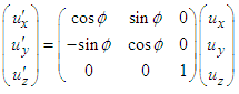 | (25a) |
 | (25b) |
from which the relativistic velocity vectors in the massive inertial frames  and
and  are written as
 | (26a) |
 | (26b) |
Figure 5 compares the Cartesian components of the transformed relativistic velocity of an event taking place in frame  (
( ) and observed in frame
  As the light source at the origin of a frame is flashed on and off rapidly, observers in both frames see a spherical shell of radiation which expands outward from the origin in all directions [2].
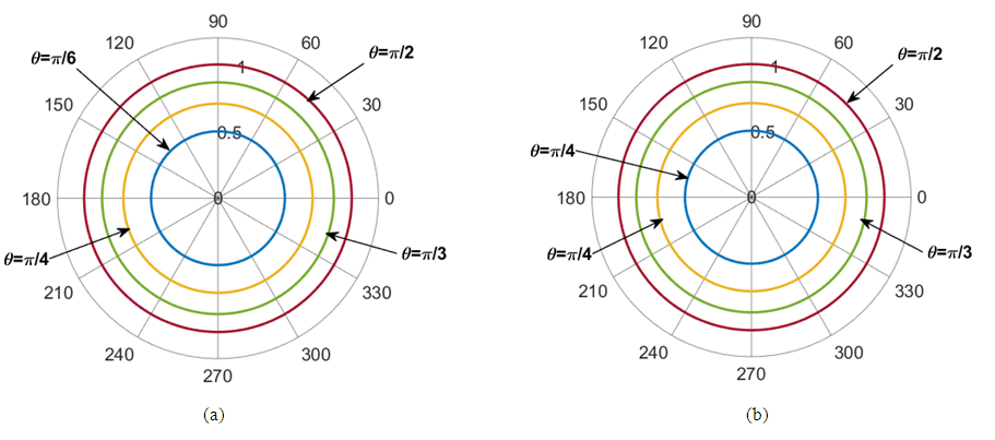 | Figure 5. Polar plot of  and and  components of components of  (a) and (a) and  components of components of  (b) plotted as a function of azimuthal angle (b) plotted as a function of azimuthal angle  for for 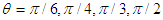 , respectively [17], [18] , respectively [17], [18] |
The upper limit for the relative speed in both frames is equal to speed of light in vacuum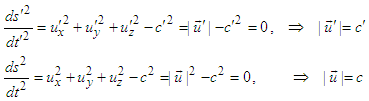 | (27) |
which proves that the speed of light is Lorentz scalar ( ) between massive inertial frames.Furthermore, similar to defining stationary position vectors
  and
and  in Fig. 4, we define stationary net force vectors
 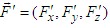 and
and 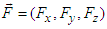 relative to unit vectors
  and
and  in the massive inertial frames
  and
and  , respectively. We then write the following matrix equations
 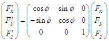 | (28a) |
 | (28b) |
from which, similar to writing Eqs. (21a) and (21b), we can write the net force vectors as | (29a) |
 | (29b) |
The scalar product of  with itself in the massive inertial frame
  leads to the scalar product of
  with itself in the massive inertial frame
 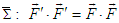 , which states that net forces have the same length
  from the origin, so vector transformation is identified as a rotation if it causes no change in vector’s magnitude [19].
4. Relativistic Invariance of Electromagnetic Fields
Considering the massive inertial frames  and
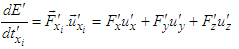
and  form a closed system in the six-dimensional spacetime, the rate at which work is done by the net force on a particle are written as [17], [18]
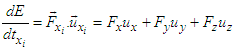 | (30a) |
 | (30b) |
where  and
and  are the Cartesian components of Lorentz force massive inertial frames
  and
and 
 | (31a) |
 | (31b) |
where  and
and  are x, y and z components of
  and
and  , given by Eqs. (25a) and (25b). Since the massive inertial frames
  and
and  form a closed system in six-dimensional spacetime, we can write the following relation for Lorentz invariance of the conservation of relativistic power law (rate of relativistic energy change) between the massive inertial frames
  and
and  [17], [18]
 | (32) |
Combining the velocity transformation matrix equations (25b) and (25a) with the conservation of power law in equation (32) we can write the following explicit algebraic equations  | (33a) |
 | (33b) |
Component by component matching both sides of Eq. (33a) and then (33b), respectively, one obtains the transformation matrix equations (28a) and (28b) for the net electromagnetic forces. Substituting Eqs. (31a) and (31b) into Eq. (33a) we write the following set of equations | (34a) |
 | (34b) |
 | (34c) |
Using Eq. (25a) for  and
and  in Eqs. (34a) - (34c), we write the transformation equations
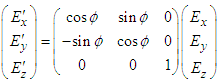 | (35a) |
 | (35b) |
which allows us to write the following expressions for electric and magnetic fields in frame 
 | (36a) |
 | (36b) |
Likewise, using Eq. (25b) for  and
and  in Eq. (33b) and following the steps in writing Eqs. (35a) and (35b), we then write the following transformation equations
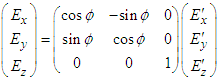 | (37a) |
 | (37b) |
from which the electric and magnetic field vectors in the inertial frame  are written as
 | (38b) |
 | (38b) |
Equations (35)-(38) are in full agreement with the first postulate of special relativity: Just as with three dimensional quantities, the relativistic vector quantities such as electric and magnetic fields should not change between two massive inertial frames under Lorentz transformation.As verification, let us consider a static point charge Q that is at rest at the origin of the massive inertial frame  which is assumed to coincide with the absolutely stationary inertial frame
  and second massive frame
  moves relative to first massive frame with uniform velocity
  . The produced electric fields in the massive frames
  and
and  are written as
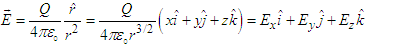 | (39a) |
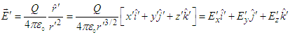 | (39b) |
where  . Using the unit vectors
  described in Eq. (22a) we can re-write Eq. (39b) as
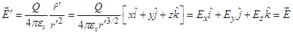 | (39c) |
which states a pure electric field in one frame appears as a pure electric field in another frame. Since observer in frame  sees the charge Q in frame
  as moving with uniform velocity
  , the magnetic field produced by charge Q in frames
  and
and  can be written as
 | (40a) |
 | (40b) |
Substituting unit vectors  from Eq. (22a) into Eq. (40b), one can write
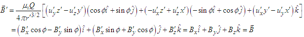 | (40c) |
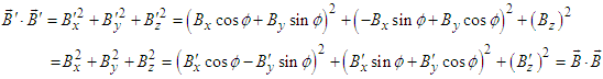
which states a pure magnetic field in one frame appears as a pure magnetic field in another one.One can easily show that scalar and vector products of electric and magnetic fields are Lorentz invariant between the massive inertial frames. The scalar products of  and
and  in the massive inertial frame
  (
( and
and  in the inertial frame
  ) are written as
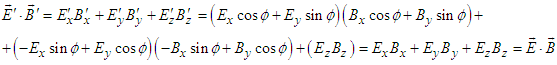 | (41a) |
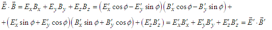 | (41b) |
which are Lorentz scalars between two inertial frames. Likewise, the scalar product of electric field  with itself and magnetic field
  with itself in the massive inertial frame
  yields
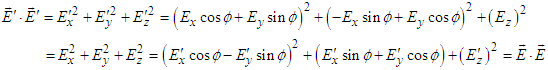 | (42a) |
 | (42b) |
which state that  and
and  (Lorentz scalar invariants). We can then write
  | (43) |
where  . Equation (43) is important for determining electromagnetic energy density.The vector product of electric and magnetic fields can be determined by using Eqs. (36a) and (36b) for
  and
and  and Eq. (38a) and (38b) for
  and
and  , which yield the following equations
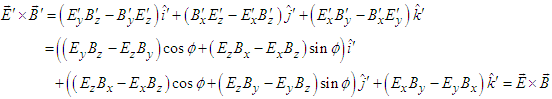 | (44a) |
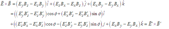 | (44b) |
which states that the vector product of electric and magnetic fields is Lorentz invariant between two massive inertial frames  and
and 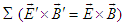 , which is essential in proving the Lorentz invariance of Poynting vector and conservation laws for charge (current) continuity equation and electromagnetic energy and momentum. This eliminates the non-invariance of electric and magnetic fields
 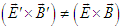 according to classical four-dimensional spacetime theory [2].
5. Relativistic Invariance of Maxwell’s Equations
Maxwell’s equation of electrodynamics must take the same form (invariant) in every inertial frame. And it is quite tedious to demonstrate this invariance explicitly by using the transformation rules in the classical four-dimensional theory of special relativity [2]. This motivated us to demonstrate the Lorentz invariance of Maxwell’s equations between massive inertial frames by using the vector transformation rules described in the previous section. In doing so, we begin with the differential forms of Maxwell’s equations in the six-dimensional massive inertial frames  and
and  , written as
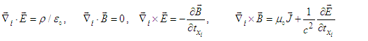 | (45a) |
 | (45b) |
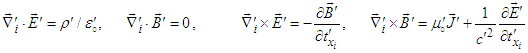
Recall that Gauss’ theorem relates the flux of a vector field  through a closed surface to the volume integral of its divergence inside the surface [20] in massive inertial frames are written as
 | (46) |
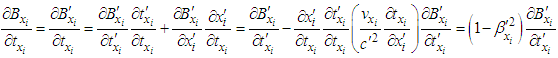
Since any scalar function, such as electric and magnetic fields, is continuous at any point in space in both frames  [21], we write the following chain rules for differential operators
  | (47a) |
 | (47b) |
 | (47c) |
where 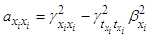 and
and 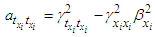 are given in Eqs. (12a) and (12b) with
  given by Eq. (14). In the following we will use Stokes theorem and chain rules to prove the Lorentz invariance of Maxwell’s equations between two massive inertial frames.
5.1. Gauss Law of Electrostatics
Since the electric field wave function is continuous at any point in space in both frames, taking  and
and  and applying the chain rule in Eq. (47a) we write
  | (48) |
where  and
and  . Matching both sides of Eq. (48) yields
  . Since
  , we have
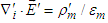
  . Consequently, covariant Eq. (44) is transformed into invariant form
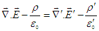 | (49) |
which is the Lorentz invariant Gauss law of electrostatics between the six-dimensional massive inertial frames  and
and  (or between four-dimensonal inertial frames
  and
and  ). Here we should keep in mind that
  and
and  defined with respect to the rest charge density
  in the absolutely steady inertial frame
  , in static equilibrium.
5.2. Gauss law of Magnetism
Since magnetic field wave function is continuous at any point in space [21], taking  and
and  and using the chain rule in Eq. (47a) we write
  | (50) |
Matching both sides of Eq. (47), one finds  , which transforms Eq. (46) to
  | (51) |
which is Lorentz invariant Gauss law of magnetism between the six-dimensional massive inertial frames  and
and  (or between four-dimensonal inertial frames
  and
and  ).
).
5.3. Faraday’s Law of Induction
Let us write the differential form of Faraday’s law of induction in Eq. (45a) in x directions of system of Cartesian polar coordinates  | (52) |
Applying the chain rule for differential operators in Eq. (47a) and (47b) to x, y, and z components in Eq. (52) for the differential form of Faraday’s law of induction we write 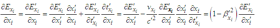 | (53a) |
 | (53b) |
where  . Combining Eqs. (49a) and (49b) side by side, we write a covariant equation
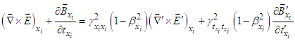 | (54) |
Matching both sides of Eq. (54), one finds 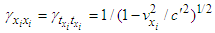 in Eq. (14) for Lorentz factor. When
  and
and  move along +x axis, 6-dimensional spacetime (3+3) becomes 4-dimensional (3+1) with
  and Eq. (54) reduces to four-dimensional invariant form
 | (55) |
which is Lorentz invariant Faraday’s law of induction between four-dimensonal inertial frames  and
and  frames in vacuum.
5.4. Ampere-Maxwell Law
We write the following forms of Ampere-Maxwell’s law (extended form of Maxwell law of induction in Eq. (45a) to include the current) in x, y and z-directions | (56a) |
 | (56b) |
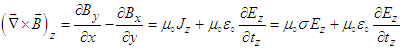 | (56c) |
where  and
and  are the conductivities in the massive inertial frames
  and
and  and
and  is the rest conductivity in the absolutely steady inertial frame
  . Applying chain rule in Eq. (47a) and (47b) to the differential form of Ampere-Faraday’s law in x, y, and z-directions and write first, second and third terms in Eqs. (56a), (56b), and (56c), we write
 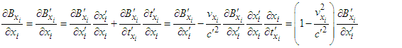 | (57a) |
 | (57b) |
Combining Eqs. (57a), and (57b) side by side and adding  and
and  on the left and right sides we write the Ampere-Maxwell law which is covariant between two massive inertial frames
  | (58) |
Matching both sides of Eq. (58), one finds  in Eq. (14) for Lorentz scaling factor, which transforms covariant Eq. (54) into the following invariant form
 | (59) |
When frames  and
and  move in one dimension (e.g., along x axis), 6-dimensional spacetime (3+3) reduces to 4-dimensional spacetime (3+1). Consequently, the Lorentz scaling factor reduces to
  and Eq. (59) then takes the following 4-dimensional invariant form
 | (60) |
which is the Lorentz invariant Maxwell law of induction between four-dimensonal inertial frames  and
and  in vacuum. Recall that
  and
and  are invariant vectors and
  and
and  are invariant scalars
  between two frames.
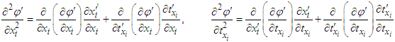
6. Relativistic Invariance of Electromagnetic Wave Equations
One of the consequences of Maxwell’s equations are the scalar wave equations [20]. Using the formula  [20], we write Faraday’s law of induction in a charge free medium
 | (61a) |
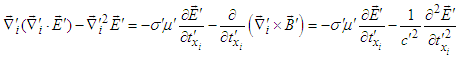 | (61b) |
where  and
and  . Using the chain rule in Eqs. (47a), (47b), and (47c) for differential operators one then writes each component of Eq. (61a) and (61b) as
 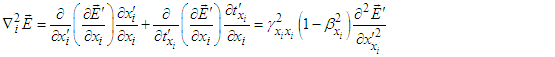 | (62a) |
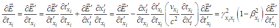 | (62b) |
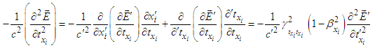 | (62c) |
In a charge free medium, covariant form of Faraday’s law between two frames is then written as | (63) |
Matching both sides of Eq. (63) one finds  in Eq. (14) for the components of Lorentz scaling factor and Eq. (63) becomes Lorentz invariant since
  and
and  are invariant vectors
  and
and  and
and  are invariant scalars
  . Maxwell’s scalar wave equation (63) for the electric field in the six-dimensional spacetime can then be written as
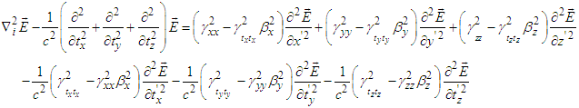 | (64) |
Component by component matching both sides of Eq. (64) then yield the components of Lorentz scaling factor given by Eq. (14). When the massive inertial frames  and
and  move along x axis, the 6-dimensional spacetime (3+3) reduces to the 4-dimensional spacetime (3+1). Lorentz scaling factor reduces to
  and Eq. (64) reduces to the following four-dimensional invariant form
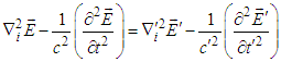 | (65) |
which is the Lorentz invariant Maxwell wave equation between four-dimensonal inertial frames  and
and  in vacuum.Likewise, using the formula from vector analysis
  [20] one writes the differential equations for Ampere-Maxwell law in frames
  and
and  in charge free medium as
 | (66a) |
 | (66b) |
where  , and
, and  . Following the steps in writing Eq. (63), we write
  | (67a) |
 | (67b) |
 | (67c) |
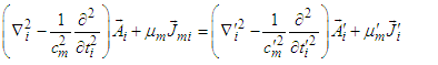
In a charge free medium, combining Eqs. (67a), (67b) and (67c) covariant form of Maxwell’s wave equation in six dimensional spacetime between two massive inertial frames is written as | (68) |
Matching both sides of Eq. (68), one finds  in Eq. (14) for Lorentz scaling factor and Eq. (68) becomes invariant. Since
  and
and  are invariant vectors (
 ) and
) and  and
and  are invariant scalars (
 ), wave equation (68) is then written as
 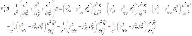 | (69) |
Component by component matching both sides of Eq. (68) yield the components of Lorentz scaling factor in six dimensions given by Eq. (14). When  and
and  move along x axis, the 6-dimensional spacetime (3+3) reduces to the 4-dimensional spacetime (3+1) and Lorentz factor reduces to
  and Eq. (69) reduces to the following four-dimensional invariant form
 | (70) |
which is the Lorentz invariant Maxwell wave equation between four-dimensonal inertial frames  and
and  in vacuum.
7. Results and Discussions
Throughout previous sections, we demonstrated that use of classical vector transformation allows one first to derive expressions for Cartesian components of relativistic invariant vector quantities, having the same length from the origin, so that a vector transformation is identified as a rotation if it causes no change in the magnitude of a vector [19]. With transformed velocity components used in the law of conservation of electromagnetic energy in a closed system, we proved that the electromagnetic fields and Maxwell’s equations and scalar wave equations are Lorentz invariant between two massive inertial frames. In this section we will give a summary discussion about the applications of the proposed theory in deriving the expressions for the relativistic invariance of the electromagnetic wave equations in the materials medium and the conservation laws of charge (current) continuity equation and continuity of electromagnetic energy and linear and angular Momentums between two massive inertial frames under Lorentz transformation.
7.1. Relativistic Invariance of Electromagnetic Wave Equations in Materials Medium
One can easily extend the six-dimensional spacetime theory to material medium wherein  and
and  by replacing the speed of light in vacuum with that in material medium as
  and
and  in the massive inertial frames
  and
and  . As an example, the covariant Maxwell’s scalar wave equations for the electric and magnetic fields in material medium between two massive inertial frames under Lorentz transformation can then be written as
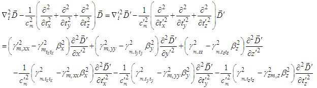 | (71a) |
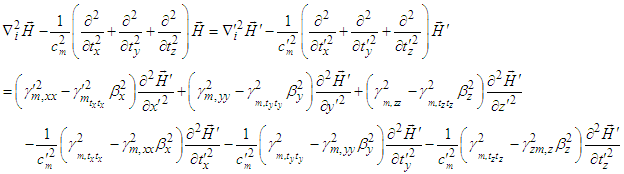 | (71b) |
where  and
and  are the Lorentz scalar dielectric constant and magnetic permittivity of a material medium in massive inertial frames
  and
and  . Here
  are the Lorentz scaling factors
  | (72) |
where  are the normalized x, y, and z components of relative velocity of the massive inertial frames
  and
and  in a material medium.We can extend the derivations carried out above to the cases in which charge and current densities are not zero. Using
  ,
,  with
with  and
and  , with
  and
and  which are defined in the massive inertial frames
  and
and  according to
 | (73a) |
 | (73b) |
 | (73c) |
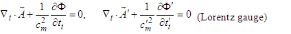
with  , respectively. Here
  and
and  are the scalar and vector potentials.
  and
and  are current densities with charge densities
 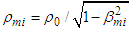 and
and  in a material medium in the massive inertial frames
  and
and  with
with  the charge density in the absolutely stationary inertial (rest) frame. We can then write the following equations
 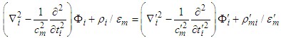 | (74a) |
 | (74b) |
which are invariant between the massive inertial frames  and
and  . Setting
  in Eqs. (68a) and (68b) one finds
  and
and  , respectively, for the velocity components.
7.2. Relativistic Invariance of Conservation Laws in Electrodynamics
Since electromagnetic waves are associated with propagation of energy and momentum in space [19], the proof of the relativistic invariance of the following relations is essential | (75a) |
 | (75b) |
 | (75c) |
where  and
and  are the energy fluxes, known as Poynting vectors, and
  and
and  are the electromagnetic energy densities,
 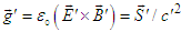 and
and 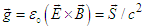 are the electromagnetic linear momentum densities and
  and
and  are the Lorentz force per unit volume exerted by the fields on the electric charge. Finally,
  and
and  are Maxwell energy-stress tensors, written as
 | (75d) |
where the indices i and j refer to the coordinates x, y and z.  is the Kronecker delta which is unity if the indices are the same (
 ) and zero otherwise (
 ). Maxwell energy-stress tensor
  is the force (stress) per unit area acting on a surface in both inertial frames with diagonal elements representing pressure and off diagonal elements are shears. In the following sub-sections we will discuss the invariance electromagnetic energy and momentum densities between two inertial frames under Lorentz transformation.
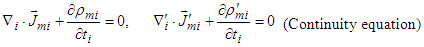
7.2.1. Current Continuity Equation
We start with employing the chain rule to differentiation in Eqs. (47a) and (47b) to write the following differential relations  | (76a) |
 | (76b) |
Side by side additions of Eqs. (76a) and (76b) allows us to write the following equation | (77) |
where  and
and  is the Lorentz scalar speed of light
  . Matching both sides of Eq. (76) yields
  in Eq. (14). When the massive inertial frames
  and
and  move in one dimension (e.g., along x axis), the six-dimensional spacetime (3+3) reduces to the classical four-dimensional spacetime (3+1). Lorentz scaling factor reduces to
  and covariant Eq. (77) is then transformed into the following four-dimensional invariant form
 | (78) |
which is the Lorentz invariant current continuity equation between four-dimensonal inertial frames  and
and  in vacuum.
7.2.2. Electromagnetic Energy Continuity Equation
Since Poynting’s theorem [20] states that the power flowing out of the volume and the time rate of increase of energy storage inside the volume equal to the total power delivered by the source to a closed electrical circuit and they can be summarized according to the following relations in the massive inertial frames  and
and 
 | (79) |
Considering  and
and  are in the same direction (
 ) using Ampere-Maxwell equation, the differential forms of Eq. (79) in the massive inertial frames
  and
and  are written as
 | (80a) |
 | (80b) |
where  [19] is used. Since
  , one can easily show that the Poynting vector is Lorentz invariant between two massive inertial frames
  | (81) |
which states that direction of light propagation is independent of massive inertial frames. Since  ,
,  and
and  letting
  or
or  and
and  or
or  , the first and second terms on the left side of Eq. (80a) in frame
  are
are | (82a) |
 | (82b) |
Side by side addition of Eqs. (82a) and (82b) allows us to write the following equation for the invariance of the continuous electromagnetic energy between two massive inertial frames | (83) |
Since  (or
(or  ) is Lorentz invariant, matching both sides of Eq. (83), one finds
 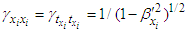 in Eq. (14). When
  and
and  move in the x-direction, 6-dimensional spacetime (3+3) reduces to 4-dimensional spacetime (3+1). Lorentz scaling factor reduces to
 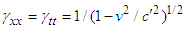 and Eq. (83) is transformed into 4-dimensional invariant form
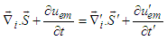 | (84) |
which is Lorentz invariant between four-dimensonal frames  and
and  in vacuum with no charge source.
7.2.3. Electromagnetic Momentum Continuity Equation
The electromagnetic field linear and angular momentums per unit volume in both frames are defined as [1]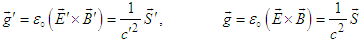 | (85a) |
 | (85b) |
Since  and
and  , so are
  and
and  , both are Lorentz invariant between the
  and
and  frames. Employing the chain rule in Eqs. (47a) and (47b) to the components of Maxwell stress tensor equation (75d) allows us to write the following relations in the
  frame
frame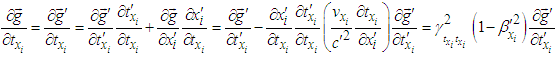 | (86a) |
 | (86b) |
 | (86c) |
Since  , addition of Eqs. (86a), (86b), and (86c) allows us to write the following equation
 | (87) |
Matching both sides of Eq. (87), one finds 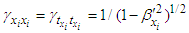 in Eq. (14). When
  and
and  move in one dimension (e.g., along x axis), the six-dimensional spacetime (3+3) reduces to the classical four-dimensional spacetime (3+1). Lorentz scaling factor reduces to
  and Eq. (87) is transformed into four-dimensional invariant form
  | (88) |
which is Lorentz invariant between the four-dimensonal inertial frames  and
and  in vacuum.
8. Conclusions
We introduced a new six-dimensional spacetime frame which allows the space and time influence of each other in the system of spherical coordinates. After satisfying Lorentz invariance of metric equation between two massive inertial frames, we derived expressions for Cartesian components of the relativistic velocity which is valid at any speed. Using the classical vector transformation method, we derived expressions for the Cartesian components of transformed relativistic velocity and electromagnetic force vectors. Considering two massive inertial frames form a closed system, we implemented the transformed relativistic velocity components into the law of conservation of energy to prove that contrary to the common belief, the electromagnetic field that appears as a purely electric (magnetic) field in one massive inertial frame, it also appears as a pure electric (magnetic) field in another massive inertial frame under Lorentz transformation. As applications of the proposed theory, we proved the relativistic invariance of Maxwell equations and scalar wave equations with and without charge and current sources, and conservation laws for the continuity of current and electromagnetic energy and momentum. Since the magnitudes of quasi-time vectors are measurable in both massive inertial frames and their Cartesian components are treated as mathematical tools, we proved that the predictions of the invariance of scalar and vector quantities in the six-dimensional spacetime frame reduce to those in the four-dimensional spacetime frame.
Data Availability Statement
This manuscript has no associated data or the data will not be deposited.
References
| [1] | Griffiths, D. J., Resource letter EM-1: Electromagnetic momentum, Am. J. of Phys., 80, 7 (2012). |
| [2] | Einstein, A., On the Electrodynamics of Moving Bodies, Annalen der Physik, 322, 10 891 (1905). |
| [3] | Lorentz, H. A., Electromagnetic Phenomena in a System Moving with any Velocity less than that of Light, Proc. Acad. Sci. Amsterdam 6 (1904). |
| [4] | Jefminko, O. D., On the relativistic invariance of Maxwell’s equations, Z. Naturforsch, 54a, 637 (1999). |
| [5] | Redžić, D. V., Comment on 'Maxwell's equations and Lorentz transformations, Eur. J. Phys. 43, 068002 (2022). |
| [6] | Sheng, X. L., Y Li, S Pu, Q Wang, Lorentz transformation in Maxwell equations for slowly moving media, Symmetry, 14, 164 (2022). |
| [7] | Anghinoni, B. G. A. S. Flizikowski, L. C. Malacarne, M. Partanen, S. E. Bialkowski, and N. G. C. Astrath, On the formulation of the electromagnetic stress-energy tensor, Annals of Physics, 432 169004 (2022). |
| [8] | Recami, E. and R. Mignani, Riv. Nuovo Cimento, 4, 209 (1974). |
| [9] | Demers, P., Canad. J. Phys.53, 1687 (1975). |
| [10] | Mignani, R. and E. Recami, Lettre al Nuovo Cimento, 16, 669 (1976). |
| [11] | Cole, E. A. B., Nuovo Cimento, 40A, 171 (1977). |
| [12] | Dattoli, G. and R. Mingani, Lettre al Nuovo Cimento, 22, 65 (1978). |
| [13] | Pappas, P. T., Lettere al Nuovo Cimento, Vol. 22. 15, p. 601-607 (1978); ibid. 25, 14 (1979). |
| [14] | Teli, M. T., Physics Letters A, 122, Issue 9, p. 447-450 (1987) |
| [15] | Guy, B., Journal of New Energy, 6, Issue 3, p. 46-71 (2002). |
| [16] | Franco, A. and Jorge, A. R., EJTP 9, 35-64 (2006). |
| [17] | Ünlü, H., Invariance of electric and magnetic fields in relativistic electrodynamics, Researchsquare.com (2022); https://doi.org/10.21203/rs.3.rs-543691/v1. |
| [18] | Ünlü, H., Special relativity in six dimensions, Journal of Asian Scientific Research, Vol 12 (2022) 188-217. |
| [19] | Kolenkow. R., An Introduction to Groups and their Matrices for Science Students, p 168, Cambridge Univ. Press (2022). |
| [20] | Reitz, J. R., F., J. Milford and R. W. Christy, Foundations of Electromagnetic Theory (3rd Ed.) Addison- Wesley Publishing Co. (1979). |
| [21] | Freeman, J. C., A new investigation into an unresolved mathematical procedure in the 1905 paper on special relativity, Physics Essays 31, 3, 310 (2018). |

 Abstract
 Reference
 Full-Text PDF
 Full-text HTML