-
Paper Information
- Paper Submission
-
Journal Information
- About This Journal
- Editorial Board
- Current Issue
- Archive
- Author Guidelines
- Contact Us
International Journal of Theoretical and Mathematical Physics
p-ISSN: 2167-6844 e-ISSN: 2167-6852
2023; 13(1): 6-14
doi:10.5923/j.ijtmp.20231301.02
Received: May 12, 2023; Accepted: Jun. 5, 2023; Published: Jun. 12, 2023

Randomizing the Bohmian Paths
 Abstract
 Reference
 Full-Text PDF
 Full-text HTML
Marcello Salis
On leave from Department of Physics, University of Cagliari, Monserrato-Cagliari, Italy
Correspondence to: Marcello Salis, On leave from Department of Physics, University of Cagliari, Monserrato-Cagliari, Italy.
| Email: |  |
Copyright © 2023 The Author(s). Published by Scientific & Academic Publishing.
This work is licensed under the Creative Commons Attribution International License (CC BY).
http://creativecommons.org/licenses/by/4.0/

Concerning the Young-Feynman interference experiment, a randomization mechanism of the Bohmian paths is proposed to reconcile the ontology of the classical particles with the “complementarity principle”. Simulations based on an elementary program code allows for results in reasonable agreement with the theory expectation.
Keywords: Bohmian Mechanics, Quantum Mechanics, Zero Point Field
Cite this paper: Marcello Salis, Randomizing the Bohmian Paths, International Journal of Theoretical and Mathematical Physics, Vol. 13 No. 1, 2023, pp. 6-14. doi: 10.5923/j.ijtmp.20231301.02.
Article Outline
1. Introduction
- The first severe criticism against the quantum mechanics (QM) conceptual framework was presented in a seminal paper by Einstein, Podosky and Rosen (EPR) that questioned the completeness of the theory [1]. According to the authors, the indeterminacy principle can be circumvented by proper tricky experiments so that, to save the QM predictions, hidden variables are to be considered in the theory. The conceptual experiment proposed by EPR considers two electrons that shares their properties by interaction, before cross measurements position/momentum take place on particles separated at distances that exceed the relativity constraint. They questioned that (in this condition) the position measurement of one particle can affect the momentum measurement on the other particle and vice versa. Bohr, in his reply to EPR, did dwell on the concept of complementary observables whose uncertainties are bounded by the quantum of action [2]. This stance just demolishes the pillar causal connection among points of a classical trajectory which is thus deprived of physical reality in the quantum realm. Inevitably, the EPR paper ushered a debate about nonlocality which was thus emerging from the prevailing interpretation of QM [3]. On this regard Bell did show that a local hidden variables theory is unable to reproduce the QM predictions, so that nonlocality is necessary to allow complementary to be manifest also in the EPR experiment [3,4]. A suggested alternative interpretation of nonrelativistic QM by Bohm aimed to recover causality through a theory reformulation (intrinsically nonlocal) in terms of hidden variables [5]. According to Bohm, the precise analysis of trajectories (initial conditions are unpredictable) can be addressed by means of the usual classical dynamics, provided a special (quantum) potential is considered which is dependent on the Schrödinger wavefunction. Predictions concerning Bohmian mechanics made for the case of matter-wave interference according to the Young-Feynman (YF) setup [6] seem to find some indirect support by experiments on photons [7], but this subject is debated and Bohmian trajectories are sometimes dubbed as surrealistic [8,9,10,11,12].The YF experiment is helpful to focus on a relevant aspect of the above mentioned debate that epitomizes the QM essence [13]. This can be well illustrated by using the Dirac-Feynman path integral approach to the problem. Accordingly, the probability that particles reach any point of a detecting screen behind the Young barrier is calculated by squaring the modulus of a (not an ordinary) integral that sums over a continuous set of complex exponentials; the corresponding phases (actions) are associated to any possible paths through the two slits [14]. Every single path has not a physical reality, as it does not define an actual particle trajectory, but the procedure evidences the essential uncertainty in connection with the crossed slit; it accounts for the complementarity of interference and “which path” information. In contrast, the Bohm description visualizes a pattern of non-crossing trajectories whose bending are indeed explained by the quantum potential that originates a non-Newtonian force on the particles. Due to their peculiarities, the whole map of the Bohmian trajectories can be separated in two sector that, against the above stance of QM, signals the slit crossed by the detected particle.The main achievement of the present work is already stated in the abstract. Here is more useful for the reader to carry out a brief presentation of the genesis of this study and its development whose byproducts explain the structure of the paper. Initially, the author interest was directed towards a better understanding of the Bohmian trajectories, bearing in mind the realistic interpretation that is recognized by a part of the scientific community. A model of the YF setup grounded on the ontology of classical particles is used as a paradigm. As presented in Section 3, it requires an elementary mathematics and allows for transparent results. Essentially, the two slits are replaced by two fixed isotropic sources that emit classical particles thus forming two associated sub-ensembles. The whole ensemble is dealt according to the Bohmian ontology whose premise is the same as for the classical motion but with a momentum restriction which, ultimately, is epistemological. Indeed, it considers the local average momentum as the actual particle property so that a fictitious potential is originated by the sub-ensemble merging. As this statistical artifact clearly goes against the realistic interpretation of the retrieved trajectories, an investigation of the statistical meaning of the Bohmian mechanics was in order. In Section 2 some recent proposals of constrained extensions of the classical statistical mechanics to quantum [15,16] are taken into account and the connections with the original Bohm's ideas are emphasized. On this ground, at the end of Section 3 the model has been extended to include the nonlocal correlation, still maintaining the basic ontology; the starting point of this extension considers the stochastic vacuum field (local) theories [17,18,19]. The model thus completed has been processed according to the Bohmian routine for the calculation of the momentum average. This is motivated by the search of those features that in the Bohmian trajectories reveal what is hidden in the standard QM. This calculation is presented in Section 4 where the comparison with the uncorrelated case is discussed. The simple analytical form of the average momentum calls for a familiar image of the flipping motion which is illustrated in Section 5 where Bohmian trajectories are shown as well. Finally, a constrained randomization of the correlated momentum flip is conjectured to account for the interference effects while maintaining the basic classical ontology and preserving the “complementarity principle”. The outcomes of an elementary program code, implemented for the simulations of the randomized motion, are compared with the theory expectations. The author remarks that this work is not to be considered the start of an alternative formulation of the QM, at least not at this stage. The theory works very well and the catalog of the relevant and well assessed formulations is remarkable [20]. Instead, the present investigation, focused on a specific problem, is motivated by the wish of a better understanding of the QM foundations that goes beyond the “shut up and calculate interpretation” [21].
2. The Bohmian Mechanics and Its Statistical Interpretation
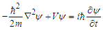
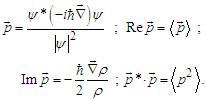
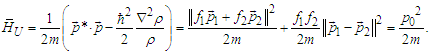
- According to the standard QM, the uncertainty principle is a necessary consequence of the probabilistic interpretation of the particle wavefunction. Instead, according to the Bohmian theory, it is only a practical limitation that concerns measurements and does not hinder a precise analysis of the particle motion [5]. For this reason, position and momentum are to be regarded as the hidden variables of the theory. Moreover, the wavefuction is to be considered as a real field responsible of a force on the particle, still maintaining the formal properties of the ensemble probability density. However, differently from other fields, a restriction of the particle momentum is to be assumed in order to match the QM predictions [5]. Briefly we recall formally the essentials of the Bohmian theory. Let us start from the Schrödinger equation, that is
 | (1) |
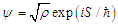 | (2) |
 and
and  are real valued functions. Substitution in eq. (1) leads to
 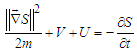 | (3) |
 | (4) |
 is interpreted as the particle momentum (the Bohmian restriction). It is also obtained
 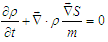 | (5) |
 is dealt with as a field coordinate and
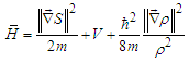
  as its conjugated momentum [5]. After the conversion in a functional form of the mean energy equation, that is
 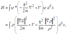 | (6) |
 | (7) |
 | (8) |
 | (9) |
 | (10) |
 | (11) |
 | (12) |
 | (13) |
 | (14) |
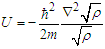
 | (15) |
 includes the quantum potential. As the model presented below imposes boundaries to the configuration domain, say
  eq. (14) is to be replaced by
 | (16) |
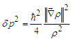
 | (17) |
 is the aforementioned random variable that satisfies
 | (18) |
 | (19) |
 | (20) |
 | (21) |
 | (22) |
3. The Model
- First consider a fixed spherical isotropic source of radius
 (radially) emitting classical particles of mass m, energy
  , de Broglie wavelength
  (be also
  ), and momentum
  | (23) |
 be the volume enclosed by a spherical surface
  of radius
  centered on the source that contains the space of interest. After every emission, a new particle is not emitted meanwhile the previously emitted particle is inside there. In order to define a density (integrable) function, it is convenient to assume that
  is covered by a particle absorber. Let N be an arbitrary number of emitted particles, large enough to fulfill any statistical requirements, then a proper time independent ensemble density can be defined as
  To give a meaning to this quantity it helps to compare locally the ensemble to a stationary fluid moving with velocity
  . Accordingly, the number of the fluid particles expected to cross a section
  in the time
  is
is 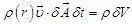 | (24) |
 is a small volume (the density is to be considered uniform). This correspondence will be used to represent the number of particles expected to cross a small volume
  throughout the experiment that is
 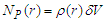 . Now fix consider two identical sources, say
  and
and  separated by
  (
( ). The absorbing sphere be centered in the median position in order to symmetrize the normalization. The sources emit exclusively one particle at time, and momenta at positions
  and
and 
 are
are | (25) |
 and
and  for particles emitted by
  and
and  , respectively. These have the same statistical properties that is
  if
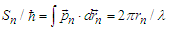
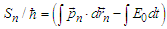
if  . The cumulative momentum within
  for the merged ensemble is given by
 | (26) |
 | (27) |
 which implies an obvious condition concerning the associated spherical angles, that is,
 | (28) |
 | (29) |
 and
and  are the angle extension of the volume projected on the plane of the Bohmian trajectories. Equation (27) in itself has not a special meaning as it results from events associated to uncorrelated sources. However, referring to the ontology of the Bohmian mechanics, according to which the actual particle momentum is defined by (27), a fictitious particle can be imagined whose trajectories (depending on the initial conditions) can be found by integrating
  | (30) |
 | (31) |
 | (32) |
 .If nonlocal correlations among particles and sources and between sources themselves come into play, a more proper calculation of the momentum average than eq. (27) is to be searched for. The nonlocality is here considered concerning how particles get their phases and how it affects their motion. The search of the average momentum will be addressed thoroughly in the next section by using the Bohmian mechanics as a statistical description of the ensemble. In the following are presented, point by point, the assumptions at the ground of the constrained momentum flip mechanism which will be used for the randomization of the Bohmian paths. 1) Classical alternatives to QM, such as stochastic electrodynamics (SED), that finds limited successes where phase is not relevant [17,18], suggest that the interaction of a particle with the zero point field (ZPF) gives its momentum a fluctuating change that vanishes on the average [19]. Here, the vacuum field is taken into account but the uncorrelated fluctuations are removed from the investigation by leaving to
  a mere geometrical meaning (the emission is radial). It is worth to point out that, due to the subsumed randomness here considered (to which is to be added a nonlocally correlated effect), there is a substantial difference with respect to the ontology of the Bohmian mechanics and the semiclassical interpretations (a brief overview in ref. [22]). Indeed, even if the particle is admitted to a precise contemporary position and momentum, without considering the observational disturbance, their instant values are meaningless in predicting the particle future, neither in retrieving its past. However, in the absence of nonlocal disturbance (see below) the average motion is considered as in the ZPF local theories.2) Unlike ZPF theories, which are essentially locals [19], it is assumed that after the particles are emitted a correlation is maintained with the sources (e.g. [23]). The latter may eventually be complex systems with internal degrees of freedom even if considered almost point-like. Therefore, it is assumed that correlated fluctuations affect the particle motion through a flip momentum mechanism (particles are conveyed toward regions where positive correlations are favored). These correlations will be defined by means of variables
  (n=1,2 labels the source that emitted the particle dealt with) that behave as
  | (33) |
 stands for the random source phase. By using symbol
  for the corresponding (internal degree) source variable and considering a large set
  of phase values presented by the source within time
  it holds
 | (34) |
 | (35) |
 is the difference between the random source phases; a random phase difference would cause the correlation to vanish. The exchange (flip) correlation for the particle can be written as
 | (36) |
 is considered as the random phase at time
  , while the particle is crossing
  , then by using
  as a particle index (phase difference is assumed to be constant throughout the experiment). The momentum flip does not occur in a deterministic way (the actual particle path is unpredictable), rather it is to be considered as a disturbance of the particle motion correlated with its own source. To illustrate the flip process with a simple scheme, it is helpful to consider particles with average momenta
  or
or  and actual random momenta
  or
or  where now random variables have possible values
  . If, for example,
  a particle found in
  with momentum
  can turn either in a fluctuation
  or
or  ; this can lead to an effective momentum flip
  . The following set of possible flips is also admitted
 3) Correlation (36) accounts for the phase difference of the fluctuating particles that enter the wavefunction representation. Given the centered isotropic dependence of the
  functions, it is not contradictory to hypothesize that the whole ZPF modes involved in forms a set showing the same symmetry (one may consider the correlations for the electric ZPF and adjust them for the scalar and centered isotropic case [17]). As the momentum flip can be regarded as a cross-exchange between the sub-ensembles, its probability is expected to depend on the (normalized) product of the numbers of involved modes pertaining the two sources. In investigating the particle motion in a plane, one can consider the only modes that are close to that plane so that their numbers are proportional to the angular extensions of the
  projection on the plane. On this ground, by taking into account eq. (29),
 | (37) |
4. The Bohmian Routine
- The Bhomian mechanics has an evident foundation which ultimately contradicts its realistic interpretation. Indeed, as a derivation of QM, it does not disentangle the two sub-ensemble (see eq. (2)) which make up the whole (ensemble irreducibility inheritance). Here one can get the point by regarding eq. (27) (note, not eqs. (25)) as the classical uncorrelated limit of the Bohmian momentum. By keeping this in mind, the two sub-ensembles are now prepared for the Bohmian routine by using wave-like functions defined for
 that is (further on densities are normalized)
 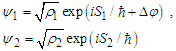 | (38) |
 that allows for
 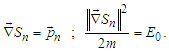 | (39) |
 | (40) |
 | (41) |
 . Indeed, after regularization of derivatives at the boundary, we have
 | (42) |
 and the small spherical surfaces of radius a, say
  , that is
  , so that
 | (43) |
 . Eventually the divergence can be removed by a suitable change of the potential definition. However, this is not necessary being this work focused on the classical interference as explained later. In this connection, it is worth to stress that the processing of the ensemble according to the Bohmian routine does not change the assumed basic ontology concerning the classical particles. On this line, conversion
  (to be considered later) is to be meant in the sense correlated-to-uncorrelated rather than quantum-to-classical. The merging of the two sub-ensembles correspond to the wavefuntion superposition which is clearly still a solution of the Shrödinger equation. The following symbols will be used:
  | (44) |
 | (45) |
 | (46) |
 | (47) |
 | (48) |
 | (49) |
 as a factor) and the corresponding potential, that is,
  | (50) |
 | (51) |
 it holds
  and
and | (52) |
 | (53) |
 is replaced by the corresponding uncorrelated average. Thus, the very difference between the two cases is reduced to the actual ensemble density. However, the Bohmian momentum convergence to (27) when
  cannot be proved by directly applying the usual mathematics to eq. (50). Instead, it can be noted that the number of density oscillations within any given small volume can be made arbitrarily large. Thus, conveniently
  can be separate in a large number of smaller equal volumes
  so that
  . Then, by assuming that inside
  the density is given by
  , it holds
  and
and  (see eq. (27)).
5. The Bohmian Trajectories and the Randomized Bohmian Paths
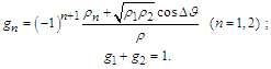
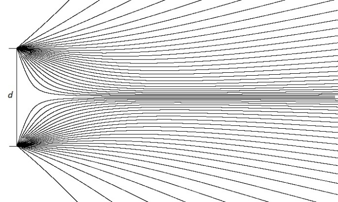
- Some pseudo-Bohmian and Young-Bohmian trajectories, whose momentum field are given by eq. (27) (uncorrelated) and (50) (correlated), are shown in Figures 1 and 2, respectively (for all the numerical calculations the used settings are: m=1;
 ;
;  ;
;  ;
;  ). In principle, a zigzag motion that closely follows these trajectories can be accounted for by the momentum flip mechanism. It is worth to detail this point in the case
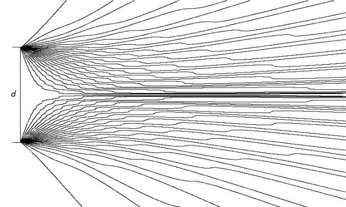
  corresponding to
  . It helps to imagine a particle advancing between two parallel walls while experiencing elastic collisions, as shown in Figure 3. The particle energy, say
  , remains unchanged but, when considering a fictitious particle that follows the projected motion along the channel direction, we see an associated reduced kinetic energy and the emergence of a “potential” that stores the lacking energy; by using eqs. (50) and (51) the momentum and the potential energy can be obtained by putting
  . This indeed may be interpreted as the results of a momentum flipping behavior
  . Things appear more concealed when considering the negative interference that occurs when
  . As
. As  , the
, the  functions not long can be used as probability factors, so that a different representation is required to handle a similar description as above. To this purpose, flip
  is considered as the actual reference flip scheme, then the average momentum is conveniently rewritten as
  | (54) |
 | (55) |
 | Figure 1. Pseudo-Bohmian trajectories obtained from integration of eq. (30) by using eqs. (25) and (27) |
 | Figure 2. Young-Bohmian trajectories obtained from integration of eq. (30) by using eqs. (25) and (50) |
 | Figure 3. Drawing of a flipping motion between walls (see text) |
 region (Figure 2). This is consistent with a fictitious kinetic energy larger than
  that, however, is to be considered a statistical bias due to the normalization. In this connection, we stress again that the realistic interpretation of these trajectories cannot be sustained due the ensemble irreducibility in the transition to the uncorrelated case. However, a possible overcome of this drawback is a weakest version of the momentum flip mechanism which is randomly distributed (with some restrictions) along the particle path. To detail this point a randomization code, that simplifies the settings presented in Section 4, is here proposed (flow chart in Figure 4). The particles are randomly emitted by the two sources and the flow chart can be symmetrically applied to them. In the following only particles emitted by source
  are considered. The momentum is determined by two variables, that is
  and
and  , so that
  . A first random number,
  , is generated to establish if a flip is to be considered or not. If
  the particle moves with momentum
  (
( ), else flips are considered but in connection with the exchange (flip) correlation. If
  only
only  exchanges are admitted. A second randomization
  is introduced for the other flips. If
  flips
flips  occurs randomly. If
  flips
flips  occurs randomly. Figure 5 shows some of the calculated paths. Figure 6 shows the calculated interference patterns at various distances from the sources and, for comparison, the theoretical density patterns. The emission of
  particles distributed within
  ; is considered and the distances are all measured in
  unit. The theoretical density has been adjusted by a factor
  where
where  stands for the distance of the detector plane from the source axis. Indeed, owing to the spreading of the real emissions in the volume, this enlarges between two close planes (considering the transverse direction with respect to the trajectory plane) as the detecting screen distance increases (the actual counts dependence on distance at the pattern center is
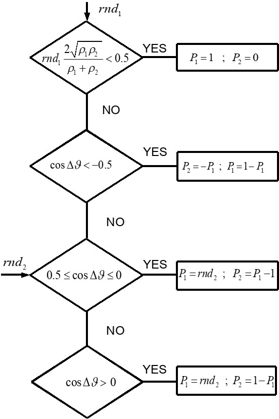 | Figure 4. Flow chart of the randomization code (see text) |
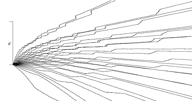 | Figure 5. Randomized Bohmian paths |
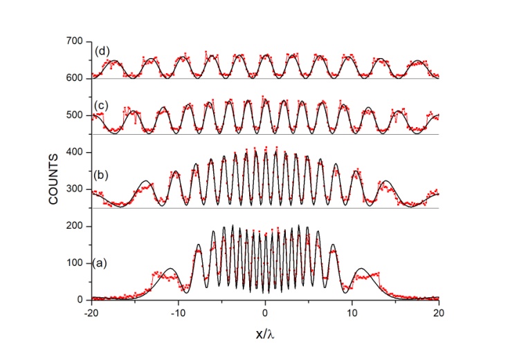 | Figure 6. Simulated (red triangles) and expected (black line) interference patterns on a plane detector at various distances from the source axis (the baseline of some data has been raised): (a)  ; (b) ; (b)  (250 counts); (c) (250 counts); (c)  (450 counts); (d) (450 counts); (d)  (600 counts) (600 counts) |
6. Conclusions
- The investigation of the Bohmian mechanics by means of a simple model of the Young-Feynman interference experiment explains its statistical character. The uncertainty concerning the actual particle path (besides the initial conditions) is an irreducible property of the experiment and cannot be resolved by the Bohmian trajectories. Nevertheless, the randomization of the Bohmian paths by using a momentum flip mechanism, induced by the interaction with the zero point field, offers a plausible representation of the real particle behavior which is also consistent with the stance of QM about the “which path” information expressed by the “complementarity principle”.