Doron Kwiat
Independent Researcher, Israel
Correspondence to: Doron Kwiat, Independent Researcher, Israel.
| Email: |  |
Copyright © 2022 The Author(s). Published by Scientific & Academic Publishing.
This work is licensed under the Creative Commons Attribution International License (CC BY).
http://creativecommons.org/licenses/by/4.0/

Abstract
The physical world has nothing to do with complex numbers and fields. These are only mathematical conveniences for describing the physical phenomena of Quantum Mechanics and Fields. Real fields and real space are the true foundations. This leads to new models for the structure of elementary particles. It is shown here that fermions are made of real coupled scalar fields. This formalism provides an explanation of familiar quantum phenomena such as interference, Planck constant and spin. Quantum mechanics should be revised, so that a direct real field interpretation will replace the current convention of complex fields.
Keywords:
Real Quantum Mechanics, Interference, Planck Constant, Spin, Maxwell Equations, Dirac Equation
Cite this paper: Doron Kwiat, Real Fields Quantum Mechanics – Imaginary Numbers are just a Mathematical Tool, International Journal of Theoretical and Mathematical Physics, Vol. 12 No. 3, 2022, pp. 79-88. doi: 10.5923/j.ijtmp.20221203.01.
1. Foreword
One can represent quantum mechanics with real fields. Using real fields (wave functions) leads to interpretation of a single particle as made of two (or more) entities represented as coupled fields [2]. Probability distributions are shown to be preserved for coupled real wave functions just as in the case of a single complex function.Assuming a string model, a double coupled string description is suggested, whereby the Schrödinger equation emerges naturally. This double-string description assumes a time-dependent tension in the strings. If the time pattern is similar for both tension and interaction, their ratio is shown to be ℏ/2. This leads to explanation of the origin of Planck's constant as the outcome of strings coupling interaction.Recent attempts [4,5] to disprove real quantum description were published, where they base their arguments on the outcome of EPR and entanglements experiments and simulations. However, one cannot come with new arguments, based on previous failed explanations. No explanation yet is given to the non-local requirements put by the entanglements assumptions. Until a logical sound resolution is given, any attempt to explain EPR and entanglement by using imaginary numbers as a true participant in physics is as valid as claims about the existence of ghosts.Complex fields in quantum mechanics are the result of hidden mechanism behind the true nature (coupled fields) of the particle, and are like a smoke screen obscuring our understanding of basic phenomena.Nevertheless, complex presentation makes our equations simpler and the results will always be the same whether real or complex approach are used. It is however important to realize that physics does not contain any imaginary numbers. This point should be stressed especially to freshmen of Physics at universities and colleges.
2. Introduction
The fact that some logical issues of quantum concepts are yet unresolved (entanglement), leads some physicists to suggest spooky concepts of complex numbers in physics [3,4,5].Though it all started in the early days of the 20th century, with the introduction of the Schrödinger equation, followed by the works of Heisenberg and others. People struggled to understand how complex wave functions can represent our reality.It is quite puzzling, in my opinion, how physicists still believe that Quantum physics has anything to do with complex numbers, and hence using Hilbert space and Hermitian operators.How can one accept an imaginary number i to participate in the description of reality?The only reason for complex numbers description of Quantum is the Schrödinger equation [1].Based on this equation the whole concept of Quantum description started in the works of Schrödinger, Heisenberg and others. The Schrödinger equation is a mathematical equation that describes changes over time of a physical system in which quantum effects, such as wave–particle duality, are significant. These systems are referred to as quantum (mechanical) systems. The equation is considered a central result in the study of quantum systems, and its derivation was a significant landmark in the development of the theory of quantum mechanics. It was named after Erwin Schrödinger, who derived the equation in 1925 and published it in 1926 [1].Schrödinger have derived his formalism by suggesting a wave equation of real fields only. It was just a matter of mathematical convenience that made him introduce complex exponentials and as he suggested, only the real part of the equations should be considered.Because of the success of Quantum formulation in describing experimental results, physicists have not bothered to pay attention to the fact that imaginary numbers do not exist in reality (not more than ghosts).In this work, a formulation of quantum fields without the use of complex numbers is given and it is shown to be equivalent to the complex fields formulation.Moreover, dealing with the real and imaginary parts separately, a single particle shows a 2-componentss behavior (and 4-components in the relativistic case). As a result, a coupled double-string description is suggested, out of which, the Schrödinger equation emerges naturally. This double-string description assumes a time-dependent decaying tension in the strings, together with a time-dependent interaction between the two strings. Interference phenomena emerges naturally for a single particle in a slot experiment. If the decay pattern is similar for both tension and interaction, their ratio is shown to be ℏ/2. Thereof, the origin of Planck constant [6-12] comes naturally.As will be shown, the Schrödinger equation and also the Dirac equation are representations of real fields, coupled together.Furthermore, under interaction with an external magnetic field, the spin emerges in the form of energy levels differences between spin-up and spin-down states.Finally, this approach allows us to observe a remarkable similarity between Dirac equation and Maxwell equations.
3. Schrödinger Equation
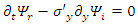
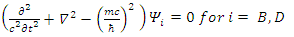
In non-relativistic quantum mechanics, a particle (such as an electron or proton) is described by a complex wave-function,  whose time-evolution is governed by the Schrödinger Equation:
 | (1) |
Here m is the particle's mass and V(x) is the applied potential. Physical information about the behavior of the particle is extracted from the wave function by constructing expectation values for various quantities; for example, the expectation value of the particle's position is given by integrating  over the entire space, and the expectation value of the particle's momentum is found by integrating
  The quantity
  is itself interpreted as a probability density function. This treatment of quantum mechanics, where a particle's wave function evolves against a classical background potential V(x), is sometimes called first quantization.
 may be written as a linear combination of the Eigen functions
  which are solutions of

 may be interpreted as the probability density of a single particle, in the ith energy state
  to be found at an interval dx around position x.The basic equation of quantum mechanics is the one particle time-dependent Schrödinger Equation:
 | (2) |
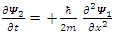
By separating Eq. (2) into real and imaginary components [2] | (3) |
the Schrödinger equation becomes: | (4) |
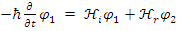 | (5) |
Where  and
and  are the real and imaginary parts of the Hamiltonian. For a time-independent classical Hamiltonian of a free particle, with mass m, it is equivalent to:
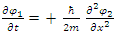 | (6) |
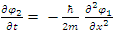 | (7) |
Applying time-derivatives on both, we obtain two decoupled equations: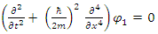 | (8) |
 | (9) |
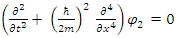
Thus  and
and  should both be solutions to the same form of wave equation, with 4th order derivative in x. Yet, the fields
  and
and  are not independent of each other, as can be seen from their coupling equations (Eqs. 6,7).It is always possible to have real operators instead of Hermitian ones and always use real space and not a Hilbert space [2]. The benefit of using complex presentation in a Hilbert space is that it makes presentations simpler. However, this comes at the cost of obscuring internal structures.
4. A Double String Analog to the Schrödinger Equation
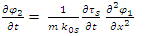
As shown [2], the two strings description leads to the following assumptions:1. A Fermion is made up of two interacting string-like entities.2. Tension in the strings is proportional to the coupling between the two strings.3. The coupling between the two strings is proportional to the amount of time the exchange lasts.One is lead to conclude, that Planck's constant  is the proportionality constant, between the total exchange (of some sort) between the two strings, and the tension in these strings.Assume a coupling between these two strings, given by a proportionality constant which will be denoted by
  The coupling is then described by the following coupled differential Equations:
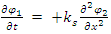 | (10) |
 | (11) |
We will also assume, without loss of generality, that the coupling constant between the two strings is proportional to the mass m. This is a reasonable assumption as we may think that the more mass, the stronger the coupling.Therefore,  and so:
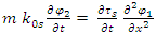 | (12) |
 | (13) |
By same reasoning, in the opposite direction, the equation will read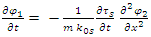 | (14) |
Assume next: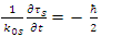 | (15) |
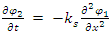
The above coupled equations now read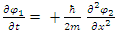 | (16) |
 | (17) |
These are the coupled real presentation of Schrödinger Equation.Equation 15 provides a physical meaning to the Planck constant, namely, independent of a particle's mass, the Planck constant  is derived from the internal quality of the real fields [7]. It represents somehow the reaction of the internal tension of the string fields to perturbations. Up to a proportionality constant,
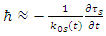 | (18) |
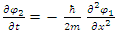
In order for this equation to make sense, one must have  as a time-dependent variable.This leads to the conclusion:
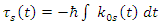 | (19) |
So, the tension in the strings is proportional to the Planck constant  and to the coupling between the two strings.This derivation of the Planck constant was made possible by the assertion of real fields coupling.
5. Probabilistic Interpretation
We remember that  is the probability density of finding a single particle at an interval dx around position x.Likewise, since
 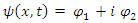 and
and  then
then | (20) |
Therefore, one may interpret this, as two interacting particles, whose probability densities  and
and  are affected by each other, and yet, together it is 1, but we cannot tell their probabilities apart.The Schrödinger equation is now interpreted as two probability density functions coupled according to Eqs. 16 and 17.The complex wave equation of a single particle, as described by Schrödinger Equation, is actually a mathematical description of two real waves functions, which, a single particle may be interpreted actually as two coupled entities.Use of the imaginary number i, and hence complex wave functions (and Hermitian operators), is just a mathematical convenience, obscuring the true internal structure of the particles.By multiplying [16] and [17] by
  and
and  respectively and integrating over x, imposing the mixed boundary conditions
  on both functions at
  it is immediately shown that (up to a normalization factor):
 | (21) |
Hence,  | (22) |
Thus, the classical coupled string system may be interpreted as a quantum mechanical single particle, described by a wave function  being a probability distribution function.This complex wave function describes a free particle of momentum
 | (23) |
When substituted in | (24) |
The result is | (25) |
Where  is a free particle Hamiltonian operator.This interpretation of a particle as made up of two real coupled strings, which tensions and interaction are connected, is equivalent to a single particle complex wave function, described by Schrödinger Equation.When the original Schrödinger Equation is used with complex wave function, the internal string-like characteristic does not show because we treat real and imaginary parts as a single entity. However, when the equation is separated into real and imaginary parts, they can be treated as two coupled strings interacting with each other, where both tension and interaction diminish abruptly, inversely proportional to time. This may be a result of weakening due to increased distance between the two strings, together with tension drop inside strings.Just like in the case of hadrons, where it is assumed their building blocks are quarks, interacting via gluons, we will assume now that leptons have some internal structure, yet to be discovered.
6. Massless and Massive Particles in the Classical Limit
Our universe is made of matter (massive particles, termed fermions with half spins with mass m>0) and of interactions between them.Interactions take place via massless entities (termed massless bosons of whole spins and mass m=0).These names are after the physicists who described their statistical qualities when considered as an ensemble. The Fermions obey Fermi statistics while Bosons obey Bose statistics. Physically, it means that fermions can never be put together at same energy state (this is related to their internal spin) while for bosons there is no limit on the number of bosons which can occupy the same energy state.When trying to show that the quantum description becomes classical, one uses  as an argument. However, such an argument is wrong.The reason is, that a particle cannot have an infinite mass. Elementary particles are limited in their mass m. It is only a collection (ensemble) of a large number of elementary particles which collectively represents a single large classical (non-elementary) mass.Thus, we cannot test the coupled equations in the limit of
  (equivalently
  ).Indeed, if we do so, we get
  | (26) |
 | (27) |
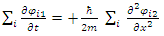
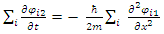
which is meaningless.The correct way of going to the classical limit  is by treating a large mass M as a collection of a large number N>>1, of elementary particles, and then sum over the coupled equations.
 | (28) |
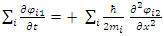 | (29) |
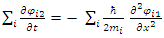 | (30) |
and for 
 | (31) |
 | (32) |
Define the collective wave functions  and
and  and thus:
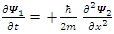 | (33) |
 | (34) |
This shows that one can no longer assume that on the limit of classical mechanics m  since all known massive particles must have finite infinitesimal mass m>0. All matter in the universe is made of elementary constituents (elementary particles). Their masses vary, but all of those that we know of have masses (rest) in the ranges of 0.511 MeV of the lightest (electron) ((≈8.6x10⁻³² Kg) to hundreds of GeV (quarks). The heaviest known is the top quark with mass of 173 GeV (≈3x10-26 Kg). Statistically, for a large N, the functions
  can be assumed non-coherent, and therefore
 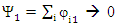 and
and 
 Thus, the quantum effect cancels out at the classical limit.Compare these masses to Planck's constant 6.582x10⁻¹⁶ eV·sec, it is of an order of magnitude of 10-3 – 10-5 [m2/sec]. So, even for the heaviest elementary particle, the Schrödinger coupled equations are valid.
7. Interference
One of the main arguments for complex probability densities is the explanation of interference.However, based on the above concept of real two coupled entities (2 fields), we show that interference can be explained with real distributions.Assume 2 slits experiment, where the separation between the two slits in the y direction is d and the particle pass through two slits.We assume now that  goes through slit 1 and
  goes through slit 2.As was shown earlier, in Eqs. 15,16, a solution for a free particle is
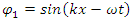 | (35) |
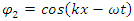 | (36) |
In two dimensions, the variations are in the y-direction while the interference plane is at a distance A in the x direction (see figure 1). | Figure 1. The interference experiment. Two slits at separation D apart, allow for two incoming particles to interfere on P(x,y) at distance A |
The fields are then: | (37) |
 | (38) |
Here we assumed x to be irrelevant in  and
and  and that the intensity of the field falls of inversely proportional to the distance.The combined field at point P(x=A, any y) is then given by
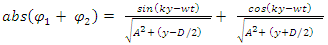 | (39) |
The resulting pattern looks like in the following (Figure 2):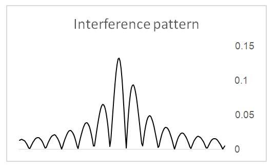 | Figure 2. An interference pattern example |
This is an explanation of interference patterns, without using complex wave functions and it is based on the identification of a single particle as made of two coupled fields. It comes instead of the duality interpretation of particles as waves-particles.Thus, even a single electron will create an interference pattern, on passage through two slits.
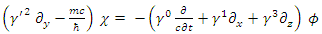
8. Dirac Equation with Real Fields
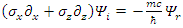
The relativistic Dirac Equation, describing a free Fermion of mass m is given by: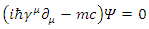 | (40) |
One may separate the Dirac operator  and the complex wave function
  into their real and imaginary parts
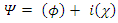 | (41) |
One will get two separate equations where  and
and  are real 4- vectors.
 | (42) |
In general, for a complex matrix operator D acting on a complex vector 
 | (43) |
 | (44) |
 | (45) |
where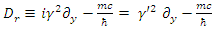 | (46) |
 | (47) |
Where 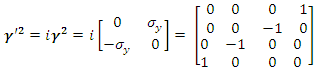 Thus,
Thus, | (48) |
 | (49) |
Since  and
and  are each a real 4-vector, they can be written as
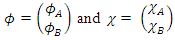 | (50) |
 are real 2-vectors each, and the real fields equations gets the following structure:
 | (51) |
 | (52) |
 | (53) |
 | (54) |
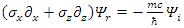
In a system where the particle is moving along the +x axis alone 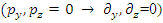 one obtains:
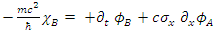 | (55) |
 | (56) |
 | (57) |
 | (58) |
These are in fact 8 different real fields, interacting via some coupling form.Define 2-vectors and the equations take the form:
 | (59) |
 | (60) |
 | (61) |
 | (62) |
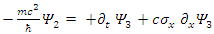
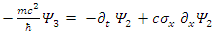
9. Eight Real Components
The  above are real 2-vectors with real components. Thus, the Dirac Equation represents actually eight equations of eight real components
 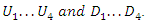 They define 4 real vectors:
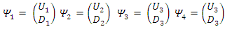 | (63) |
The pairs  and
and  are coupled as is evident from Eqs. 59-62.By applying a time derivative to the first equation of each pair and using the second of each pair (Eqs. 59-62), one obtains:
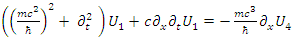 | (64) |
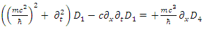 | (65) |
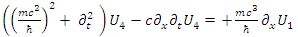 | (66) |
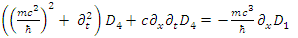 | (67) |
 | (68) |
 | (69) |
 | (70) |
 | (71) |
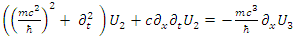
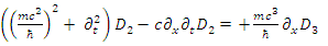
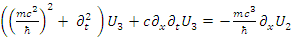
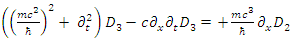
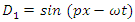
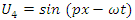
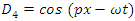
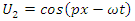
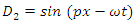
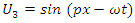
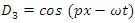
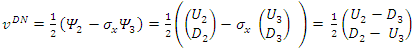
These establish the couplings: U1 ↔ U4, D1 ↔ D4 and U2 ↔ U3, D2 ↔ D3.
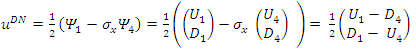
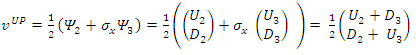
10. Solving the Equations
A possible solution to these coupled differential equations will be of the form: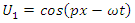 | (72) |
 | (73) |
 | (74) |
 | (75) |
 | (76) |
 | (77) |
 | (78) |
 | (79) |
When inserted in the 8-componenents equations and solving, one obtains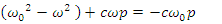 | (80) |
 | (81) |
 | (82) |
 | (83) |
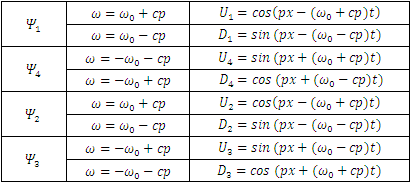
The fields are then (Table 1):Table 1. Summary of the possible suggested solutions
 |
| |
|
With  where
where  is the x component of the momentum.When boosted to the rest system
  we can see that for all components
 | (84) |
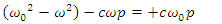
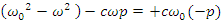
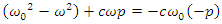
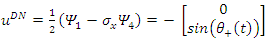
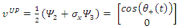
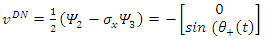
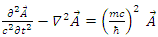
Solving this equation by setting  or
or  shows that all components of this fermion at the rest frame, are oscillating at a rate given by
  At such high oscillating rate, the spin cannot be determined apriori, and depends on the random outcome of the instance of measurement. As a result, the measured spin outcome is random, with equal probabilities for being up or down.The necessary conclusion is that each particle with spin, must have a definite time dependent spin. This spin oscillates at a fixed rate
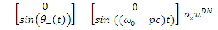
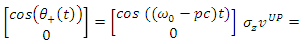
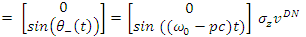
 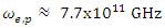 for an electron.Hence, pending on the instance of creation we will get a certain result – up or down. It looks like a mixture of states merely because the temporal resolution is insufficient.Since in an electron-positron creation, both are created simultaneously, their spins will be correlated.Thus, there are two particles states involved. One, denoted by (+) precessing around the x axis in a positive right direction, and the other, denoted by (-), precessing around the x axis in the opposite (left) direction:
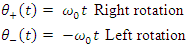 With
With  At a boosted system, where p=0:
11. Spin under a Magnetic Field
We will use now the results for a boosted system, that is, we move with the massive elementary particle. Define  and
and  4-vectors as follows:
 | (85) |
 | (86) |
 | (87) |
 | (88) |
To find their spin state in the +z direction we apply  to find:
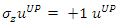 | (89) |
 | (90) |
 | (91) |
 | (92) |
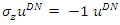
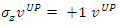
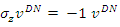
This verifies the fact that the measured eigenvalues of these states are indeed ±1. It represents two eigenfunctions of spin-up and spin-down for the u solution and two eigenfunctions of spin-up and spin-down for the v solution.Similarly, to find their spin state in the +x direction we apply  The interaction between the fermion and the magnetic field B is given by
 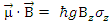 where g is the g-factor of the fermion. Under a magnetic field
  the change in energies of the above states is given by
 | (93) |
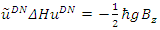 | (94) |
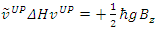 | (95) |
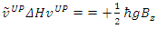 | (96) |
This demonstrates that in the presence of a magnetic field, there exist two spin states (up and down) for  and two spin states (up and down) for
  The energy difference between two states is given by
 | (97) |
The energy difference between the two states is independent of time and of their spatial location along the x-axis.The two states are time-dependent and position-dependent, yet their spin does not change with time and in space: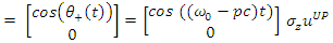 | (98) |
 | (99) |
 | (100) |
 | (101) |
As is obvious from the above description of states, both electron and positron, when created simultaneously, will have their spins corelated.The up state gives always a spin +1 but, as evident, the state itself varies with cos() between  to
to  .The rate of change is (for electron)
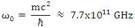 Obviously such high oscillations rate is beyond our current detection capabilities.We notice, that the spin state is an energy state. We differentiate between spin up and spin down by their energies compared to their state without magnetic field interaction. So, as long as the energy state remains unchanged, the phase is irrelevant.Recall that
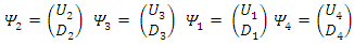 | (102) |
Therefore: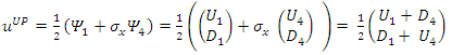 | (103) |
 | (104) |
 | (105) |
 | (106) |
Notice, that prior to the interaction with an external magnetic field, one cannot say anything about the spin of the electron. All we know is that it is made up of 4 real fields  and
and  that can be combined mathematically into 2 complex vector fields
  and
and  These can in turn be combined to form 2 different states with eigenvalues +1 or –1 when operated upon with the
  operator. Likewise, there is another particle which is made up of 4 real fields
  and
and  that can be combined mathematically into 2 complex vector fields
  and
and  . These can in turn be combined to form two different states with eigenvalues +1 or –1 when operated upon with the
  operator. It is the interaction with a magnetic field that reveals the difference between an up state and a down state.All above calculations were made using real fields alone. No need for complex representations.
12. Other Fermions
As can be seen, solution to the Dirac Equation results in 8 real constituents altogether. They create 4 coupled pairs. Two coupled pairs connect in either symmetric or anti symmetric states, to create a spin-up or a spin down fermion.An electron is made of symmetric (spin-up) and antisymmetric (spin down) combinations of U2 D4 D1 U4. A positron made of symmetric (spin-up) and antisymmetric (spin down) combinations of U2 U3 D3 D2.Dirac Equation describes the electron and the positron. But there are other fermions such as muon, tau, proton, neutron and quarks. Are they Dirac particles as well?Irrespective of their assumed internal structure (3 quarks), the free nucleons can be described by the classical Schrödinger equation with their kinetic energy term described by their momentum p and rest mass m. Therefore, by transferring to the relativistic equation, one must have the Dirac Equation for nucleons as well. Moreover, any massive particle must answer the Dirac Equation. Hence, all massive elementary particles must be spin 1/2 particles.Obviously, when dealing with compounds of elementary particles, this no longer is true. The reason of course is that a compound of a large number of elementary particles is an assembly of wave functions which result in an average tending to zero. (See earlier discussion about massless and massive particles and classical limit).Based on the string interpretation, we can describe the internal couplings U1 ↔ U4, D1 ↔ D4, U2 ↔ U3, D2 ↔ D3 by some exchange mechanism that binds them together.The fermions are then the result of combing pairs of such couple in either symmetric or antisymmetric states. This will explain then the spin half characteristics of these fermions.
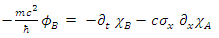
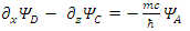
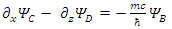
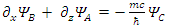
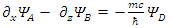
13. Similarity between Dirac and Maxwell Equations
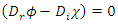
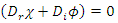
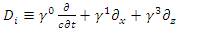
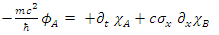
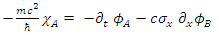
The symmetry between Maxwell equations and the Dirac equation were discussed already by others [14,15,16]. There, a slightly generalized classical Maxwell were considered. The group-theoretical properties of this equation, its symmetries and its unitary relationship with the Dirac equation were investigated. It was shown there, that slightly generalized classical Maxwell electrodynamics can describe the inner atomic phenomena with the same success as relativistic quantum mechanics can do.Due to the unitary relationship with the Dirac theory, the electric charge is a conserved quantity in the same sense as in the Dirac’s model. It may be defined similarly to the Dirac theory or may be derived from it on the basis of unitary relationship [16].In the following this symmetry will be approached by the use of real fields in the Dirac equation.Recalling that  and
and  and decomposing
  into
into  and
and  are real 4-vectors), the Dirac equation becomes
 | (107) |
or, | (108) |
Which leads (after separation of real and imaginary parts) to: | (109) |
 | (110) |
 | (111) |
 | (112) |
This leads to the conclusions:1. The real and imaginary components are coupled.2. Both real and imaginary parts have 4 components eachSince both  and
and  are made of 2 real components each, there are 4 components altogether.
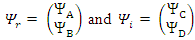 Eqs. 134-137 can then be formulated in terms of 8 real coupled fields as follows:
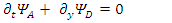 | (113) |
 | (114) |
 | (115) |
 | (116) |
 | (117) |
 | (118) |
 | (119) |
 | (120) |
These equations hint to some connections between the possible states of the fermion.Applying  to Eqs. 117-120 results in
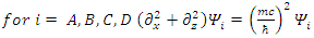 | (121) |
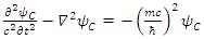
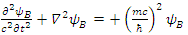
There are apparently 4 constituents of the Dirac particle. The above two groups of differential equations show the coupling that exists between the constituents.There is a clear asymmetry in the Dirac equation, as there is a difference between the y coordinate and the x-z coordinates. This is in contradiction with the expected isotropic spherical symmetry of the Fermions and the need of the results to be independent of the coordinate system.By applying second time derivative, Eqs. 113-116 can be written as | (122) |
 | (123) |
These can be combined to give: | (124) |
 | (125) |
We thus see, that Dirac equation becomes 4 real waves equations. Each is a Klein-Gordon (KG) equation. Since the solutions to the Klein-Gordon equations are well known, we can conclude and say, that the Dirac relativistic Fermion is actually a 4 Fermions equation. These 4 Fermions are of same mass m.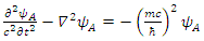 | (126) |
 | (127) |
 | (128) |
 | (129) |
If now  and
and  are the mirror functions of
  and
and  , respectively, then
  , and
, and 
 Therefore
 | (130) |
 | (131) |
 | (132) |
 | (133) |
In other words, we have four possible KG solutions. Two solutions (A, C) with positive energy term and two solutions (B, D) with negative energy term. These equations show that the four states can exist independently of each other.Suppose we define two 3 components vector fields [13] | (134) |
 | (135) |
With  some arbitrary vector field.The fields
  and
and  satisfy:
 | (136) |
for the y component.Same relationships exist for | (137) |
 | (138) |
Leading to | (139) |
Again, for the y-component.This may hint to some internal structure of a Dirac fermion, being made of some interacting electromagnetic fields.Let us look at the electromagnetic field vector  It satisfies Maxwell's equations
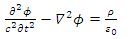 | (140) |
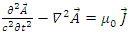 | (141) |
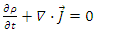
Assume the Dirac charged fermion has an internal current density and hence an internal vector potential.This particle has an internal electric charge distribution  and create an internal current
  Because of current conservation and the definition of the vector potentials we have
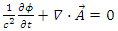 | (142) |
 | (143) |
Suppose now that the current density is proportional to the vector potential:  and
and  Then the above conservation equations are always satisfied.This leads to:
 | (144) |
 | (145) |
which have the same form as the Dirac 4 real fields, Eqs. 44-47.If | (146) |
 | (147) |
and 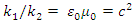 Then,
Then,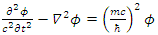 | (148) |
 | (149) |
In other words, the four Dirac fields  are the electromagnetic vector potential fields,
  provided that the current densities
  are related to the electromagnetic fields
  by Eqs. 146, 147 through the constant
  .There are no external electromagnetic fields, so these are confined electromagnetic fields which create the fermion and give it its mass m.Note though, that in order to keep with the signs as required, the currents
  and
and  must be symmetric with
  and
and  about their spatial coordinates, so that their spatial derivatives change signs accordingly.
14. Conclusions
We assumed all quantum fields, to be real wave-functions in real space, acted upon by non-Hermitian operators. it was shown that both Schrödinger and Dirac equations describe the behavior of both non- relativistic and relativistic Fermions. The picture of interacting strings, leads us to conclude that both Schrödinger and Dirac equations describe some exchange mechanism between coupled strings.One may therefore re-consider our view of leptons as being elementary particles. Just like Hadrons are assumed to be made of quarks interacting via gluons and confined.This interpretation can explain interference in a similar manner to the explanation by standard quantum mechanics of complex wave functions.Moreover, this approach provides possible explanation to the Planck constant.Spin emerges naturally by inspecting the energy levels under the interactio of the reaql fields with an external magnetic field.Physics has nothing to do with neither complex space nor complex fields. Complex Quantum mechanics is just a mathematical convenience which obscures the true essence of elementary particles.
References
| [1] | Schrödinger E, "An Undulatory Theory of the Mechanics of Atoms and Molecules", Physical Review, Vol 28(6), December 1926. |
| [2] | D Kwiat, "The Schrödinger Equation and Asymptotic Strings". International Journal of Theoretical and Mathematical Physics, Vol 8 (3) 2018. |
| [3] | Matthew F. Pusey, Jonathan Barrett and Terry Rudolph, "On the reality of the quantum state", Nature Phys 8, 475–478 (2012). |
| [4] | Renou, MO., Trillo, D., Weilenmann, M. et al. "Quantum theory based on real numbers can be experimentally falsified". Nature 600, 625–629 (2021). |
| [5] | MC Chen, C Wang, FM Liu, JW Wang, C Ying, "Ruling out real-valued standard formalism of quantum theory" Physical Review Letters, 2022 |
| [6] | Steiner L.R., History and progress on accurate measurements of the Planck constant, Reports on Progress in Physics, vol. 76 (1), (2013). |
| [7] | D Kwiat, "Derivation of Planck's Constant from Two Strings Coupling". International Journal of Theoretical and Mathematical Physics, 10 (2) (2020). |
| [8] | D Kwiat, "Planck’s Constant—A Result of Two Strings Coupling", Journal of High Energy Physics, Gravitation and Cosmology Vol.8 No.4, (2022). |
| [9] | Anton A. Lipovka, "Planck Constant as Adiabatic Invariant Characterized by Hubble’s and Cosmological Constants", Journal of Applied Mathematics and Physics, 2, 61-71, (2014). |
| [10] | Ulrich E. Bruchholz, "Derivation of Planck’s Constant from Maxwell’s Electrodynamics", 2009 Progress in Physics Volume 4. 2009. |
| [11] | Evans, M. Derivation of the Evans Wave Equation from the Lagrangian and Action: Origin of the Planck Constant in General Relativity. Found Phys Lett 17, 535–559 (2004). |
| [12] | Donald C. Chang, "Physical interpretation of the Planck’s constant based on the Maxwell theory". Chin. Phys. B Vol. 26, No. 4, (2017). |
| [13] | D Kwiat, "Dirac Equation and Electron Internal Structure", International Journal of Theoretical and Mathematical Physics, 9 (2): 51-54, 2019. |
| [14] | Krivskii, I. Yu. . "Dirac Equation and Spin 1 Representations, A Connection with Symmetries of the Maxwell Equations". Theoretical and Mathematical Physics Vol. 90, 265-276 (1990). |
| [15] | V. Simulik. "Relativistic Quantum Mechanics and Field Theory of Arbitrary Spin, Nova Science, New York, 2020, 343 p., Chapter 1. |
| [16] | V. M. Simulik, I. Yu. Krivsky, "Relationship between the Maxwell and Dirac equations: Symmetries, quantization, models of atom", Reports on Mathematical Physics 50(3): 315-328 2002. |

 Abstract
 Reference
 Full-Text PDF
 Full-text HTML