Phillip Frank, Hermann Rohte
University of Vienna, Austria
Copyright © 2021 The Author(s). Published by Scientific & Academic Publishing.
This work is licensed under the Creative Commons Attribution International License (CC BY).
http://creativecommons.org/licenses/by/4.0/

Abstract
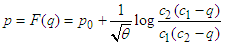
For all equations of transformation which correspond to one-term linear groups, there are three types for which the amount of contraction does not depend upon the direction of motion. Furthermore, only one type has a contraction of lengths as a consequence; namely the Lorentz transformation [Equation (1)]. The two other types, the Galilei and Doppler transformations [Equation (2) -- (129)] the lengths are left unchanged. For the Lorentz transformation the velocity of light in all moving systems has the same value,  . For the Doppler transformation only for propagation in one particular direction occurs when the velocity of light is infinite.
Keywords:
Lorentz Transformation, Gallilei Transformation, Special Relativity
Cite this paper: Phillip Frank, Hermann Rohte, The Transformation of Spacetime Coördinates from Resting to Moving Systems, International Journal of Theoretical and Mathematical Physics, Vol. 11 No. 4, 2021, pp. 141-152. doi: 10.5923/j.ijtmp.20211104.02.
1. Introduction
The transformation equations which link the spacetime coördinates  of a system at rest with those of a system
  moving with velocity
  (with constant magnitude and direction) have attained great importance in current physics. Therefore it is worthwhile to examine carefully the physical or other reasonable assumptions that are actually required to obtain the structure of the equations of transformation. According to the theory of relativity they are given by the Lorentz transformation. In familiar notation, if one represents the velocity of light in vacuo by the symbol
  and chooses the coördinate systems such that at time
  they coincide, and then one of them moves in the
  -direction:
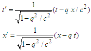 | (1) |
In the limit  [** with
  **] we obtain the familiar Galilean transformation:
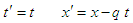 The usual standard derivation of equation (1) originates from work of A. Einstein [1], which rests essentially upon the following assumptions: •
  If
If  is the value of the velocity of light with respect to a system at rest, it must also follow that the velocity of light has that same value with respect to all systems moving in uniform straight line motion with respect to thee rest system. This assumption is equivalent to the mathematical requirement that the relations (2) follow directly from the equations of transformation.
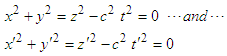 | (2) |
•  The equations of transformation should be linear and homogeneous in the coördinates; the corresponding coefficients can then depend only on the relative speed
  .•
.•  If
If  , the transform should be mapped into its inverse (that is, Eq. (1) with
  expressed in terms of
  •
•  The contraction factor,
  in Eq. (1), which alters lengths depending on the motion, should depend only on
  .We wish to show that the number of requirements can be considerably reduced, and in particular the one that is presumably the most important assumption. That is, we eliminate
  , the requirement that the velocity of light is the same in resting and moving systems.We can obtain Eq.(1) with only the following assumptions:• A. The transformation equations labeled by
  considered as a variable parameter form a linear, homogenous group,
  .• B. The length contraction factor should depend only on the absolute value of
  .The group property of the transformation equations in A must necessarily be required if these equations are to be valid for all velocities
  . If these equations do not form a group, then the composition of the two transformations, that is the transformation to a moving system with the aid of an intermediate system, would lead transformation equations with a structure quite different from that of the original system.First we will determine the most general transformation consistent with requirement A. By specializing we obtain everything that also satisfies condition B. We obtain either the simple form of the equations which contain no contraction factor, or else the Lorentz transformation (1). The first case is to be identified with a new type of transformation (we call it the Doppler transformation), and obtain the Galilei transformation (2) as a special case.We have already done a portion of the analysis of these assumptions in the paper [2] “Über eine Allgemeinerung des Relativätsprinzips und die dazu gehörige Mechanik”. For example we obain the most general form of the formula for addition of velocities under condition A. [3]W. v. Ignatowsky [4] has already made an attempt to reduce the Einstein assumptions to a smaller number, If one takes into account explicitly all the tacit assumptions that one has made, one can render the content as follows: he avoids assumption (
 ) (constancy of the light velocity), retains our assumptions, and also keeps Einstein's assumption (
 ). By combining at once all the propositions, he does not obtain the most general transformations satisfying A, and therefore obscures the special position of the Lorentz transformation in this general framework.This work proceeds as follows. At the outset we make the restrictions
 because the analysis of the equations is fairly easy, and avoids needless difficulties that might otherwise arise. Therefore we consider only the transformations of
  and
and  .In Chapter I we briefly review the concepts and rules of transformation groups. [5] In Chapters II and III we apply these results to the transformations specified by condition A. In Chapter IV we introduce a parameter
  [** the group parameter **] which has the characteristic of a velocity, and leads immediately to the addition theorem for parallel velocities. In Chapter V we give an example of these developments. In Chapter VI we finally calculate the form of the most general transformation satisfying condition A., and in particular the contraction factor as a function of the velocities considered in IV. Finally, in Chapter VII we impose condition B. and obtain all systems that satisfy our requirements.
2. Chapter I
1. Let  be three variables, where
  signifies the rectilinear coöordinate of a point
  in the
  plane, with
  a parameter. Also let
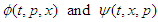 | (3) |
be two single-valued continuous and differentiable functions of the three arguments [6] for which the Jacobian (functional determinant)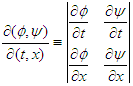 | (4) |
does not vanish identically, nor do the factors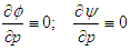 | (5) |
vanish identically. From these two equations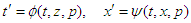 | (6) |
if the parameter  has a fixed value, each ordered pair
  corresponds to a second pair
  . This correspondence is called a transformation, which is represented by
  , a pointwise mapping of the
  plane onto the
  plane.In effect, we map a point
  into the point
  , using the same underlying coöordinate system for each of them.2. The parameter
  may pass through all numerical values, or vary over a restricted interval, so that we have an infinite set
  of transformations
  , for which each has a particular value corresponding to the parameter
  . This is called a one parameter continuous family of transformations.Let
  denote a second transformation in the set
  , which belongs to parameter
  and transforms
  into
into  , so that
 | (7) |
We eliminate  from equations (6) and (7), to obtain the equations
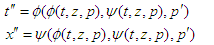 | (8) |
which represent the transformation  which takes
  directly into
  and is the product of the two transformations
  and
and  . That is,
 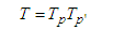 | (9) |
where the ordering of the factors in the product corresponds to the order in which the transforms should be performed. In general,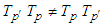 | (10) |
That is, the combination of transformations  does not satisfy the commutative rule3. The product of two transformations in the set
  as represented by
  will, in general, not lie in the set
  . However, if the product of two arbitrary transformations in
  also lies in
  , then the transfomations is
  are said to possess the group property. In that case:
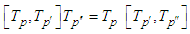 | (11) |
That is, the product of three (and arbitrarily many) factors obeys the associative law.If  is a group; that is, if T belongs to
  , Eq. (8) must have the form
 | (12) |
where | (13) |
is a function of  and
and  alone,The transformations in
  form a group
  when the following conditions are met:• A. The transformations of
  obey the group composition property.• B. There is a particular parameter
  , for which
 | (14) |
The transformation  corresponding to this parameter
  , which satisfies the equations
 | (15) |
leaves the pair  unchanged, and is called the identity transformation.• C. For each transformation
  there is a second member of
  for which in either order of combination there results the identity transformation
  . These two transformations are called inverse transformations, and we call
  the inverse transformation to
  , so that
 | (16) |
The inverse transformation to  is obtained if one solves Eq. (6) for
  , which is always possible, since the functional determinant never vanishes identically. If the inverse transformation
  to
to  corresponds to the parameter
  , which depends only on
  , then we make the identification
 | (17) |
According to (13) the two values  and
and  thereby satisfy the equation.
  | (18) |
Then  is a one-parameter group, which consists of an infinite number of transformations.4. If we consider
  in Eq. (18) as a variable that is to be transformed and
  as a parameter (or inversely) then eqn (18) defines a one parameter family of transformations, labeled by the transformed value
  , which constitute a one-parameter subgroup of
  .5. If
  is an infinitesimal parameter, which corresponds to the parameter
 | (19) |
it yields a change which is infinitesimally close to the identity transformation.It is called an infinitesimal transformation of the group which transforms the point  into an infinitely near point
  , with these coördinates.
 | (20) |
where | (21) |
if we set | (22) |
In the equations (21), which define the infinitesimal transformations, it is permissible to substitute  for
for  , where
  denotes a non-vanishing constant, without in any essential way altering the structure of the group
  . If one regards two infinitesimal transformations connected in this way as identical then every one parameter group contains only a single infinitesimal transformation. Inversely, each arbitrary infinitesimal transformation (21) induces a definite one-parameter group. The finite equations (6) can be obtained by integration of the simultaneous system
 | (23) |
with the initial conditions | (24) |
6. Let us now think of  as a function of
 | (25) |
and thereby obtain a curve  in the
  plane. It transforms under (6) into a curve
  that satisfies the relation
 | (26) |
If we set | (27) |
then | (28) |
We introduce the abbreviated notation | (29) |
for the transformation in eq. (6) related to  . For
. For  we use (14) to obtain
 | (30) |
Therefore | (31) |
that is, | (32) |
For  we obtain
 | (33) |
and make an infinitesimal transformation of 
 | (34) |
or, briefly, | (35) |
Eqns. (6) and (28) together form a one-parameter group  of transformations, which convert the variables
  into
into  . This group
  is called the first extended group. Its infinitesimal transformation is given through Eqns. (21) and (34), and one gets the finite equations (6) and (28) by integration of this system:
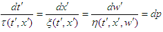 | (36) |
with the initial conditions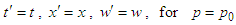 | (37) |
3. Chapter II
7. Let us choose a coördinate system  containing a fixed direction, the
  axis, and with a fixed origin
  . On the
  axis we place observers with a clock at each point.Let us consider the motion of a material point
  along the
  -axis, with corresponding readings of the clocks lying along the
  -axis, forming the ordered pair
  , over a particular set of observers. This motion is specified by eqn. (25) and the velocity is given by the first equation in (27).If we interpret the quantities
  as coördinates of a point in the
  plane, for each point in
  there is a point
  in space-time, which lies in a system
  of space-time coördinates. The complete motion of
  is represented by a continuous path of space-time coördinates; that is through the curve
  , eqn. (25), which is called the world-line for this motion. The velocity
  at time
  is equal in value to the tangent to the world-line at point
  . The corresponding motion of
  lies along a straight line.8. Along with the system
  we consider with the same straight line another simple infinite set of systems
  (that is, of length and time measurements), each of which has a definite value of the parameter
  , such that different values of
  correspond to different
  systems. An arbitrary point
  in the system
  with space-time coördinates
  has coördinates
  in each system
  , which is dependent only on
  and
and  . That is, the space-time coördinates of
  which are, respectively,
  and
and  and are connected by equations of the form (6). We call the quantities
  the space-time coördinates of
  as measured in
  . The infinite number of values of
  , lead to an infinite number of values of
  , which arise from
  from the one-parameter set
  of transformations. [7]If we compose two transformations of the set
  using the transformations (6), we go from system
  to a second system
  and then again through equation (7) to a third system
  , so that the transformation (8), which goes directly from
  to
to  , should also lie in the set
  . That is, the set
  should possess the group composition property.Furthermore, we assume that the original system
  , which also lies among the systems
  , corresponds to the parameter value
  , so that for
  equation (6) must become equation (15); thus the set
  contains the identity transformation.Finally we require that each transformation also has an inverse in
  , so that for each
  there is a parameter
  such that equation (1) is satisfied. Thus the transformations form a one-parameter group
  , which we describe as follows:The transformations (6), which take the original space-time coördinates
  in the system
  into coördinates
  in the system
  , form a one-parameter group with the parameter
  .9. In order to specify the group
  more precisely, we make the following additional assumptions.A. Each motion which is uniform with respect to a system
  at rest is also uniform with respect to a system
  in motion. Therefore when the world line of a curve
  in
in  is a straight line, the world line curve
  must also be a straight line. That is, the transformations of the group
  must generate straight lines from straight lines. The only transformations of this sort are projections, [8] that is, those whose equations (6) are of the following special form:
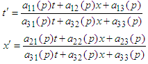 | (38) |
The group  is then called a one-term projective group. [** It is at this point that the explicit expressions which ultimately lead to the Lorentz transformations enter the development of the theory **]B. Each space-time point which has finite coördinates
  must also have finite coördinates
  in the system
  . It follows [9] that in equation (38)
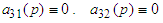 | (39) |
If we make the replacements | (40) |
for  and
and  , (38) can be rewritten in the form
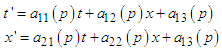 | (41) |
The transformations (41) which leave infinite regions of the  plane invariant, are called affine; the group
  is then called affine or general linear.C. Finally the specification of the origin must be the same in all systems, so that if
 it should follow that
 Therefore
 | (42) |
so that equation (41) becomes the following: | (43) |
These transformations (6) for  are linear homogeneous functions of
  with coefficients that depend only on the parameter
  . The group
  is called a one-parameter linear homogeneous group. Its transformations map infinite straight lines in the
  plane into straight lines and leave the origin invariant. [10]It is hardly necessary to remark that the coefficients
  cannot be chosen arbitrarily, but must satisfy certain conditions for the transformations to form a group. Determination of the form of these coefficients is given below.
4. Chapter III
10. We can summarize all of our assumptions concerning the transformations (6) again as follows: The transformations (6) which take the original system  into a system
  , form a linear homogeneous group with the single parameter
  .We shall consider Eq. (43) subject to the initial conditions at
  , which correspond to the identity transformation:
 | (44) |
For  , with
  small, we obtain
 | (45) |
When we define the quantities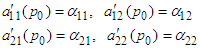 | (46) |
Then the equations for an infinitesimal transformation [see eqns. (19) -(22) in 5.] appear in the form | (47) |
so that for the linear homogeneous group (43) we obtain | (48) |
The coefficients  may then be chosen arbitrarily; only their mutual relation is relevant. As a result there are
  infinitesimal relations (47), and each one generates a particular one-parameter linear homogeneous group (43).11. If we consider a given transformation in
  , with the parameter
  held fixed, by differentiation of (43) we obtain the equations
 | (49) |
From this it follows that the differentials  transform just like the finite quantities
  ; thus the two pairs
  and
and  are co-gradient systems.From Eqn (49) it follows that
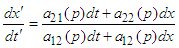 | (50) |
so that from (27)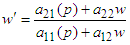 | (51) |
This equation, which gives the transformation of velocity  into
into  , now replaces eq. (28) and represents Equation (43), the first extended group
  . Of special importance is the situation in which the linear group requires that
  is a function only of
  and
and  , and not dependent on
  and
and  . From (34) and (48) we obtain the infinitesimal transformation of velocity as
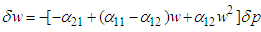 | (52) |
which implies that the function  in (35) is independent of
  and
and  . This infinitesimal transformation changes the velocity so that
  goes into
  . It remains unchanged only when
  | (53) |
This occurs for velocities  which are roots of the quadratic equation
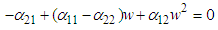 | (54) |
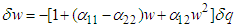
They remain the same under an infinitesimal transformation, and we will verify directly that [see the conclusion of No. 12.] that each finite transformation also leaves the group  unchanged. In the succeeding we shall call these the exceptional velocities.Note that the case of rest (
 ) is not an exceptional velocity, which means that necessarily
 | (55) |
Because of condition (55) the case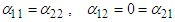 in which (54) is identically satisfied, implies the possibility that every velocity
  is an exceptional velocity, is excluded. In every other case we have two exceptional velocities, which we call
  and
and  ; namely
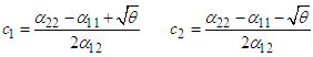 | (56) |
where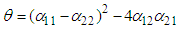 | (57) |
The symmetric combinations of the roots  and
and  are
are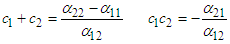 | (58) |
and with these relations the infinitesimal transformation (52) can be brought into the form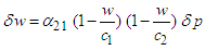 | (59) |
in which the significance of  and
and  as the exceptional velocities is immediately apparent.
5. Chapter IV
12. In order to obtain the finite forms (48) and (51) of the extended group  , which is generated by the infinitesimal transformations (47) and (52), we proceed to integrate the simultaneous system (36)
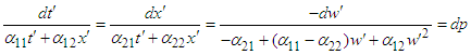 | (60) |
with the initial conditions (37). In the interim we shall apply this method to Eqn. (51) for the velocity  in order to determine its transformation. It will be useful to note that
  depends only on
  and
and  but is independent of
  and
and  . This implies that in (60) we can separately consider the equation
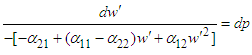 | (61) |
with the initial conditions  | (62) |
The direct integration, then has the form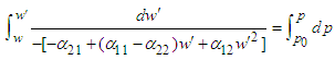 | (63) |
In evaluating the integral on the l.h.s. we take into account that the two exceptional velocities  and
and  are the zero points of the denominator. The result can be written the form
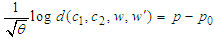 | (64) |
where  represents the double relation of the four values of
  ; i.e the expression
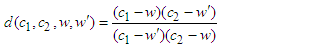 | (65) |
According to (61) we finally obtain | (66) |
Let us solve for  to obtain
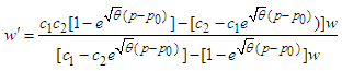 | (67) |
which is the finite equation for the transformation of the velocity [compare (25) and (51)]. Furthermore we can set  and
and  equal to their values in (56). [11]Observe that in equation (67) the two exceptional values
  and
and  are indeed unchanged, and thus have the same value in every system obtained by the finite group transformation. If we replace
  , respectively, it follows that
 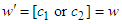 for every value of the parameter
  .13. The systems
  , which we introduced in II.8, are to be connected to the original system
  , which we described as at rest, by motions with constant velocity
  . Then since the system
  corresponds to a particular parameter
  as well as to a definite velocity
  , there must be a relation between
  and
and  , which we write as
 | (68) |
so that the parameter  appears as a function of the velocity
  .If we use the velocity
  instead of the parameter
  in equations (43) and (51) in virtue of (68), the group
  is not changed essentially when
  is considered as the new group parameter.To define the parameter
  and also to determine the form of the function
  , we make the following requirement:If the point
  is moving with respect to the resting system
  with velocity
  , since the system
  also moves with velocity
  with respect to
  , then
  has velocity
  in
in  .Thus we require that the pair
 | (69) |
should obey equation (64), so that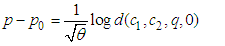 | (70) |
This yields the explicit form of the function 
 | (71) |
We use this expression in (67) to obtain the equation of transformation of the velocity  as
as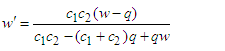 | (72) |
or, according to (58)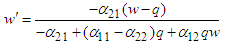 | (73) |
Furthermore, it follows from (71) that the parameter  as the identity transformation corresponds to velocity
  . The system
  at rest therefore singled out among the systems
  , as the one which moves with velocity
  .14. Let us from now on consider the velocity
  as the group parameter, and set
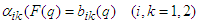 | (74) |
From (43) and (51) we obtain the equations | (43a) |
and | (51a) |
which now defines the group  . If we set
  in (51a) then necessarily
  . Moreover this identity follows for every value of
  :
: | (75) |
If we now consider the new equations (43a) and (51a) as the basis for the group  , then the value
  yields the identity and the value
  the corresponding infinitesimal transformation. The equivalent result can be regarded as following from Eqn. (47) because the introduction of the new parameters
  can alter the values of the coefficients
  but not their mutual relations -- and only these relations are relevant.With our normalization of the group parameters, the coefficients
  acquire specific values, whereas previously only their relative behavior was fixed. In fact it follows from (45) and (46) that
 and therefore if we use the identity (75), with
  , and neglect terms of second order we obtain
 which means that
  | (76) |
since  . Thereby, the coefficient
  , which was previously constrained only by the inequality (55), is determined exactly.According to (44) and (46) we obtain for the new coefficients
  in (43a) and (51a) the relations
 | (44a) |
and | (46a) |
Finally we insert the value (76) in equations (47) and (52) we obtain for the infinitesimal transformations of the group 
 | (47a) |
and for the infinitesimal transformation of velocity 
 | (52a) |
or, from (59)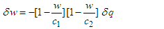 | (59a) |
The finite equation (73) for the velocity becomes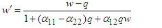 | (73a) |
and from (57) directly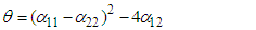 | (57a) |
15. When we consider (73a) with the parameter  and a second transformation of the same sort involving
  , we obtain
 | (77) |
From the group property of our transformations, it follows that  must be generated from
  with some value
  of the group parameter; that is
 | (78) |
where the parameter  is a function of
  and
and  .In order to determine this function, it is only necessary to write the composition of (73a) and (77) explicitly
 or
or | (79) |
By comparison with (78) it follows then | (80) |
This equation, through which the parameter group  of our groups
  and
and  is given, [12] expresses the addition theorem of group velocities for the system
  , which moves with velocity
  with respect to
  , which itself moves with velocity
  with respect to system
  .If equation (77) is taken to represent the inverse transformation, then
 so that the resulting transformation (78) should represent the identity, and
  . It follows from (80) that if we denote the parameter value of the inverse transformation by
  , we obtain
 | (81) |
so that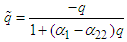 | (82) |
If we put this value in place of  in (72), the inverse equation for (77) becomes
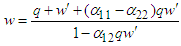 | (83) |
as one can also verify directly by solving (78a) for  .The formula (83) shows that
  obtained from
  and
and  in exactly the same way as is obtained for
  from
from  and
and  -- an analogy that clarifies the kinematic meaning of equations (80) and (83).
6. Chapter V
16. Before we consider the general form for the finite group  , we shall exhibit as examples of the preceding development the two special one parameter linear homogeneous groups (2) and (1) mentioned in the introduction: these are the Galilei and Lorentz transformation groups.The coefficients
  of group (2), the Galilei transformations, are
 | (84) |
from which it follows that at  they reduce to
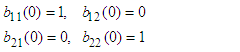 | (44b) |
in agreement with (44a). Furthermore, it follows from (84) that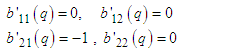 | (85) |
and therefore from (46a) that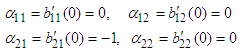 | (46a) |
so that equation (76) is satisfied. For the infinitesimal transformation (47a) and (52a) we obtain | (47b) |
and | (52b) |
Finally from (57a) we obtain | (57b) |
so that the two exceptional velocities are equal to one another, and in particular | (86) |
while the finite transformation (73a) of velocities becomes | (78b) |
For the group (1) of Lorentz transformations, the coefficients  are given by
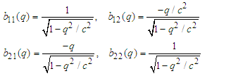 | (87) |
where for  they again lead to equations (44a). For the derivatives
  we find
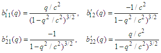 | (88) |
and from this it follows that (46a) implies that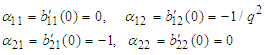 | (46c) |
so that equation (76) is also satisfied. Equations (47a) and (52a) yield the infinitesimal transformations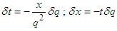 | (47c) |
and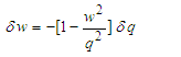 | (52c) |
so that for the exceptional velocities for  and
and  we obain the values
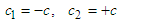 | (89) |
Now from (57a) 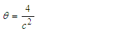 | (57c) |
and therefore we finally obtain from (73a) the finite transformation of velocity  in the form
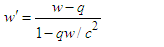 | (73a) |
7. Chapter VI
17. Now let us proceed to set up the general equations for the one parameter linear homogeneous group  ; that is, the determination of the coefficients
  in (43a).From equivalence of the two equations (51a) and (73a), it follows from their consistency that the four coefficients
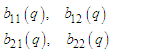 | (90) |
and the four quantities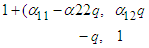 | (91) |
must be proportional. Moreover the proportionality factor can depend only upon  . We write it as
  , [** In the succeeding we write
  in many appropriate places in the text; this replaces
  which through oversight appears in many expressions **] so that
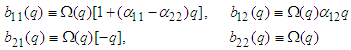 | (92) |
where in addition the identity (75) is satisfied. By inserting the values (92) into equation (43a), we obtain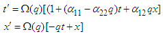 | (93) |
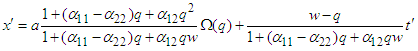
where the function  is unknown.18. The kinematic interpretation of the factor
  can be inferred by means of equation (93), but we still have to determine its form. If we consider a point
  which moves along the
  -axis with constant velocity
  and is located at position
  at time
  , its motion is described by the equation
 | (94) |
In order to determine the equation of motion of  with respect to a system
  moving with velocity
  with respect to system
  , let us solve equation (93) for
  and
and  , to obtain
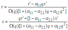 | (95) |
for the inverse transformation of (92), and insert the expressions (95) into (94). We thereby obtain Therefore, when we solve this equation for
 | (96) |
or | (97) |
where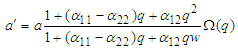 | (98) |
is the value of  at
at  and
and  is the velocity of
  in the system
  , as given by (73a).Let us consider two points
  and
and  which have space time coördinates
  and
and  in the resting system
  , and which move with the same constant velocity
  . At time
  the locations of
  and
and  are given by
 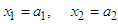 so that the equations of motion of these two points with respect to
  are
are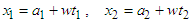 | (99) |
In the system  moving with velocity
  with respect to
  , the equations of motion are
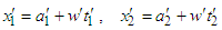 | (100) |
where  and
and  are the space-time coordinates of
  and
and  in the system
  . Furthermore, from (98),
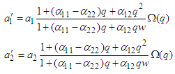 | (101) |
where  is the velocity of the points in the system
  , as given by (73a).The two points
  and
and  , which move with the same velocity
  along the
  -axis, can be thought of as end points of a rigid rod, with length
  in the
  system. [** The measurement of lengths is entirely compatible with the principles of special relativity; however the idealization of the existence of perfectly rigid bodies leads to paradoxes, and therefore these models of physical objects must be excluded. **] Therefore at equal times
 subtracting these two equations in (99), we obtain
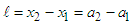 | (102) |
We can determine the length of the rigid rod  , as measured in the system
  , when at the same times
 we again obtain by subtracting the corresponding equations
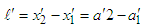 | (103) |
Then from (101) and (102)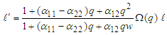 | (104) |
Finally if we also assume that the slab is at rest in the system  , that
  ; then in accordance with (69) it moves in the system
  with velocity
  . It follows from (104) that
 | (105) |
In other words the function is the factor with which the length  of a rod at rest in system
  must be multiplied to yield its length
  in the system
  , with respect to which it is also at rest, when
  is moving with velocity
  relative to
  . The factor
  is called the contraction factor.19. In order to determine the specific analytical form of
  , we use the parameter
  in ther transformation (93) which converts the pair
  into the pair
  , together with a second transformation from the group
  :
: | (106) |
This transform converts  into
into  using the parameter
  . From the group multiplication property of the transformations, it follows that the resulting transformation, which converts
  into
into  has the form
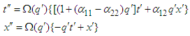
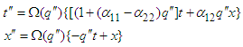 | (107) |
where the parameter  is is given by equation (80) as a function of
  and
and  .If we actually join the two equations (93) and (106) together, and use equation (80), we obtain
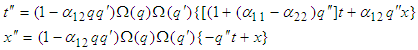 | (108) |
by comparison with (107) this implies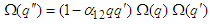 | (109) |
Therefore from (80):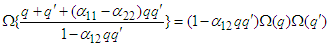 | (110) |
This is a functional equation, through which it is possible to determine the structure of the function  . For this purpose we differentiate (110) with respect to
  and then set
  , to obtain
 | (111) |
But from the last equation in (92) so that the contraction factor
  according to (44a) and (46a) also satisfies the conditions
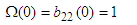 | (112) |
and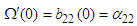 | (113) |
by means of which we obtain the differential equation | (114) |
with the initial conditions (112). It follows from (114) that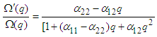 | (115) |
and therefore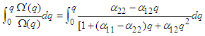 | (116) |
If we calculate the integrals on both sides of (116) and solve the resulting expression for  , we find the following expression for the contraction:
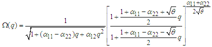 | (117) |
which in fact also satisfies condition (113).Thereby the final equations (98) for the general one parameter linear group, which through the infinitesimal transformation (47) is generated under conditions (55), is completely determined.20. For the Galilei group one finds from (46b) | (117a) |
and for the Lorentz group from (46c)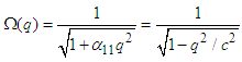 | (117b) |
in agreement with equations (2) and (1).
8. Chapter VII
21. Let us now proceed to analyze and investigate the constraints imposed by condition B., where the three continuous parameter groups which, through equations (93) and (117) give the contraction  , result in an even function of the velocity
  ; that is, properties which are independent of the direction of the
  -axis.For this situation it is necessary and sufficient that the odd order derivatives of
  vanish at
  ; in particular
 | (118) |
We shall calculate the quantities  . The first two are given through equations (112) and (113); we obtain the rest most simply by repeated differentiation of equation (114). The results, when we set
  , are
, are | (119) |
 | (120) |
It follows that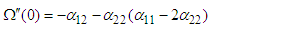 | (121) |
and | (122) |
It follows from the first equation (118), taking into account equation (113) that | (123) |
and then from (122) that | (124) |
Equations (123) and (124) must be necessarily satisfied if the transformation equations for the contraction should obey requirement B. We will soon see that the requirements (123) and (124) are also sufficient conditions22. There are three sub-cases that satisfy equation (124):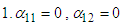 | (125a) |
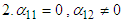 | (125b) |
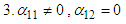 | (125c) |
Each of these sub-cases corresponds to a particular type of transformation equation which satisfies the basic conditions A. and B.For the first alternative, using equation (98) and taking into account the connection together with (117) and (117A), gives the Galilei transformation. The second alternative, as seen from equation (93) with (117) and (117A), gives the group of Lorentz transformations.23. The third alternative leads to a group which has not yet been considered. It follows from equation (117) together with (123) and (125c) that | (126) |
and from equation (93) that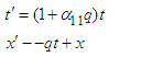 | (127) |
The exceptional velocities have the values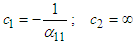 | (128) |
since these are the roots of the quadratic equation (54), where the coefficients obey the conditions (76), (123), and (125c). The transformation (127) then has the form | (129) |
The transformation of time in these equations can be given a physical interpretation, just as Einstein has given for the Lorentz transformation. At time  a light ray originating at the origin and moving in the positive
  -direction moves with velocity
  . When a body moves with velocity
  , then light moves with velocity
  in the resting system. If we now wish the velocity of the light ray with respect to the time of the moving system is also
  , we can accomplish this by changing the rate of the clock in a ratio proportional to the fraction
  , so that for the moving body the time is
  , given by
 as is given by the first equation (129). This time adjustment corresponds to the Doppler principle; and therefore we will call the transformation (129) the Doppler transformation. The Doppler transformation is essentially different from the Lorentz transformation, in that for bodies moving with velocity
  the same time prevails at all points; there is no space-time variation for them, and what is more important: if we restrict the direction of production of a light ray to the
  -direction, then all bodies moving in this direction possess the same light velocity
  (we take
  ); consequently light rays produced in the negative
  -direction are not in alignment with all moving bodies.When
  is an exceptional velocity, then
  is not one as well. According to equation (128) this would only be true for
  , or
, or  , but then we would recover the Galilei transformation.However, in the case of Lorentz transformation, because of equation (56) together with equations (76), (123), and (125b). we obtain
 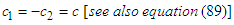 We can summarize the results of our investigation as follows:Of all transformation equations that correspond to a one-parameter linear homogeneous group, there are three types for which the behavior of contraction does not depend upon the direction of motion in absolute space. Only one of these types yields a meaningful contraction of length; namely the Lorentz transformation [equation (1)]. The two other types, the Galilei transformation and the Doppler transformation [equation (2); especially (129)] leave the lengths unchanged. In the Lorentz transformation the velocity of light has the same value
  for all systems moving in arbitrary directions. For the Doppler transformation this occurs only when the transformation lies in one direction; for the Galilei transformation only when the velocity of light is infinite.
ACKNOWLEDGEMENTS
The original German language manuscript was obtained from the source BNFGallica: utilisaton.commerciale@bnf.fr.
Translators Comments
The following article is translated from the original German text:"Uber die Transformation der Raumzeitkoordinaten \\ von ruhenden auf bewegte Systeme” von Philipp Frank und Hermann Rothe. Ann. d. Phys. Vol 34 (series 4) 1911. pp 825-855.This paper was of special importance in understanding the Lorentz transformation in the context of the special theory of relativity. Namely, only these two requirements were made:(1) inertial invariance and(2) that the product of two boosts in a given direction yielded a boost in the same direction.It was shown that there are only two (consistent) possibilities: (a) a Galilean Transform or (b) a Lorentz Transform. It was not necessary to assume that the velocity of light is identical in all inertial frames. Note: deviations in translation are marked by [** **].Thomas Erber and Porter Johnson*; Department of Physics; Illinois Institute of Technology; Chicago, Illinois, USA.
References
| [1] | A. Einstein, Jahrb. d. Rad u. Elektr. [4] (1897) p.411 ff. A more careful analysis of Einstein's derivation is found in the work: Ph. Frank, Sitzungsber. d. k. Akad. d, Wiss in Wien. Math-phys KL [118], Abt. IIa (1909) p. 421 ff. |
| [2] | Ph. Frank and H. Rothe, Sitzungberichte d. k. Acad. d. Wiss. in Wien, Kl. 119, Abt. IIsa, p. 615 ff, 1910. |
| [3] | Previous reference, equation (12) and the following unnumbered equation. |
| [4] | W. v. Ignatowsky, Berichte d. Deutsch. Phys. Ges. p. 788 ff and Arch. f. Math. u. Phys, 17 p. 1 ff 1910. |
| [5] | We have consistently employed the elementary theory of group representations as described by S. Lie and G. Scheffers, Lectures on Continuous Groups (1898) Leipzig. |
| [6] | The three variables  must necessarily be of limited ranges over the manifold being considered, which belongs with the coördinate system must necessarily be of limited ranges over the manifold being considered, which belongs with the coördinate system  . . |
| [7] | The remainder of Chapter II is unnecessary for understanding this work, and serves only to make condition A. plausible. |
| [8] | S. Lie and G. Scheffers, loc cit p 32, Theorem 2. |
| [9] | Loc cit, p.57-58, Law 11. |
| [10] | S. Lie and G. Scheffers, loc cit p. 184. |
| [11] | Note that equations (64), (66), and (67) are independent of the  sign in front of sign in front of  . Namely, if we replace . Namely, if we replace  by by  in (56), the two invariant velocities in (56), the two invariant velocities  and and  are exchanged, and the equations remain unchanged. are exchanged, and the equations remain unchanged. |
| [12] | If one considers the original parameter  of the group, which for example appears in (67), then equation (13) gives the group parameter of the group, which for example appears in (67), then equation (13) gives the group parameter  . . |

 Abstract
 Reference
 Full-Text PDF
 Full-text HTML