Jody A. Geiger
Department of Research, Informativity Institute, Chicago, IL, USA
Correspondence to: Jody A. Geiger, Department of Research, Informativity Institute, Chicago, IL, USA.
| Email: |  |
Copyright © 2021 The Author(s). Published by Scientific & Academic Publishing.
This work is licensed under the Creative Commons Attribution International License (CC BY).
http://creativecommons.org/licenses/by/4.0/

Abstract
It has been a long-standing goal in physics to present a physical model that may be used to describe and correlate the physical constants. We demonstrate, this is achieved by describing phenomena in terms of Planck Units and introducing a new concept, counts of Planck Units. Thus, we express the existing laws of classical mechanics in terms of units and counts of units to demonstrate that the physical constants may be expressed using only these terms. But this is not just a nomenclature substitution. With this approach we demonstrate that the constants and the laws of nature may be described with just the count terms or just the dimensional unit terms. Moreover, we demonstrate that there are three frames of reference important to observation. And with these principles we resolve the relation of the physical constants. And we resolve the SI values for the physical constants. Notably, we resolve the relation between gravitation and electromagnetism.
Keywords:
Measurement Quantization, Physical Constants, Unification, Fine Structure Constant, Electric Constant, Magnetic Constant, Planck’s Constant, Gravitational Constant, Elementary Charge
Cite this paper: Jody A. Geiger, Measurement Quantization Describes the Physical Constants, International Journal of Theoretical and Mathematical Physics, Vol. 11 No. 1, 2021, pp. 29-59. doi: 10.5923/j.ijtmp.20211101.03.
1. Introduction
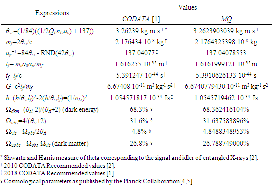
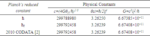
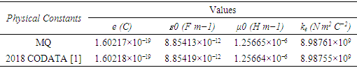
We present expressions, their calculation and the corresponding CODATA [1,2] values in Table 1.Table 1. CODATA and MQ expressions for the physical constants
 |
| |
|
Calculations start with measurement of the magnetic constant. Along with defined values, this provides a CODATA value for the fine structure constant 7.2973525693 10-3 which may be considered a physically significant guide for the remainder of the calculations. The count distance nLr=84.6005456998 corresponding to blackbody radiation may be resolved with twelve digits of physical significance knowing its approximate count nLr=84 of lf. The value of lf is not needed in that the value of nLr is a mathematical property of discrete counts. The product, QLnLr is calculated using the Pythagorean Theorem QL=(1+nLr2)1/2-nLr. Such that QL+nLr describes the hypotenuse of a right-angle triangle of sides nLr=1 and some count nLr of the reference lf, then QLnLr=0.49998253642 and with this we can resolve θsi kg m s-1. θsi also describes the angle of polarization with respect to the plane of entangled X-Rays [3] and has no units when describing properties of the universe. With θsi, the defined value for c and the fundamental expression lfmf=2θsitf – resolved from Planck’s Unit expressions [6] – we resolve fundamental mass mf and the Planck form of the inverse fine structure constant αp−1. Using Planck’s expression along with measures for the ground state orbital a0 and mass of an electron me – both measures from the 2018 CODATA – we resolve fundamental length lf. And we continue with the resolution of the gravitational constant G, Planck’s reduced constant ħ and those values typically resolved with ΛCDM. The electromagnetic constants involve several concepts and will be discussed later.Notably, the fundamental expression is provided without explanation. The difference between the Planck and electromagnetic descriptions of the fine structure constant are not discussed. Our goal, initially, is to demonstrate the approach. The formulation, physical significance and explanation of each expression is the purpose of this paper.Of the many descriptions of phenomena, it may come as a surprise that there are few expressions that describe discrete behavior as a count of some fundamental measure [4]. Perhaps one of the first and most notable is Planck’s expression for energy, E=nhv. That said, the property of discreteness exists with respect to several phenomena (i.e., those radii that identify orbits where there is a highest mean probability of electrons being fundamental to atomic theory). In that we describe phenomena mathematically in relative terms, it follows that the property of discreteness carried within such expressions is disguised beneath the macroscopic definitions that make up much of classical mechanics.In this paper, we reduce the classical nomenclature to a more fundamental set of terms that incorporates a description of discreteness. We accomplish this by taking the existing classical nomenclature and incorporating the concept of counts of fundamental measures to accommodate the possibility of discrete measure. However, measure is not to be assumed countable or discrete. As such, we refrain from introducing biases, provide an accommodating nomenclature and then apply that nomenclature to existing phenomena to learn if there exists a physically significant correspondence.We begin with three notions: Heisenberg’s uncertainty principle, the universality of the speed of light, and the expression for the escape velocity from a gravitating mass. Each describes a bound to measure, respectively a lower bound, an upper bound, and a gravitational bound, the latter being needed to incorporate the mass bound with respect to the prior two. Using the new nomenclature, we identify three properties of measure: discreteness, countability, and the relationship between the three frames of reference. After resolving minimum count values for length, mass, and time, we then resolve physically significant values for the fundamental measures, matching values in the 2010 CODATA [2] to six digits. Importantly, we learn that measure with respect to the observer is discrete, whereas measure with respect to the universe is non-discrete. This difference allows us to resolve the constants and the laws of nature.We identify this presentation as the Informativity approach – a term that describes the application of measurement quantization (MQ) to the description of phenomena. The nomenclature we call MQ. There are several papers that apply MQ to describe phenomena in disciplines such as: quantum mechanics, classical mechanics (including gravity, optics, motion, electromagnetism, relativity), and cosmology [7–11]. Nevertheless, a discussion of the physical constants is prerequisite to a thorough understanding of MQ. For that purpose, the first half of this paper is a review of concepts established in prior papers [10,11].Foremost, we introduce a consequence of discrete length; discrete units of length limit the precision with which objects can be measured relatively. Importantly, the property of discreteness is not only intrinsic to measure but also to the laws that describe what we measure. The methods section focuses on correlating this to expressions that describe nature.Moving forward, we describe how discrete measure skews the measure of length, an effect like that of Special Relativity (SR). Not accounting for this effect reduces the precision of expressions, especially those that include Planck’s constant. It is for this reason that the Planck Units have largely been considered coincidental and without physical significance.Once completing the expressions for the fundamental measures, their relationship, and a quantum interpretation of gravity, we commence Section 3 describing the fundamental constants resolving their values and physical significance using only the MQ nomenclature (i.e., lf, mf, tf, and θsi). It is here that we part with the self-referencing definitions that have deadlocked modern theory. Specifically, we redefine the physical constants not as functions of one another (i.e., ɛ0=1/μ0c2) [1], but as functions of the fundamental measures. Several examples include elementary charge, the electric and magnetic constants, Coulomb’s constant, the fine structure constant, and the gravitational constant.With new definitions for gravitation and electromagnetism written in a shared and physically distinct nomenclature, we establish a physical reference with which to resolve what differentiates them. There are five expressions that describe their difference: two describe an observational skew in measure, one describes the fine structure constant as a count while another describes elementary charge using only fundamental units. The final term – a mathematical constant – describes what separates the energy of a particle from a wave. Although described entirely as a function of mathematical constants, the particle/wave duality is difficult to physically ascertain. The correlation, we admit, lacks the purity of classical concepts such as distance, velocity, and elapsed time.From a broader perspective, the correspondence between geometry and physical expression becomes even more important. Its correspondence arises in so many expressions that we feel compelled to identify such descriptions as consistent with the phrase, ‘the metric approach’, short for geometric or a consequence of the geometry of a phenomenon. We do not mean to emphasize the mathematical properties of this correspondence as to say that such properties follow the same consistency as that of SR. In this light, we present physical constants, such as the fine structure constant and Planck’s reduced constant as counts of one fundamental measure. Importantly, the metric approach is not distinct from classical mechanics. Nevertheless, many of the physical constants are described as counts of one fundamental constant to be discussed at the outset in Section 2.5.Finally, using MQ to describe the physical constants resolves several discrepancies between classical theory and measurement. For one, the precision limits of Planck’s unit expressions are resolved. Furthermore, disagreement between Planck’s expression for the ground state orbital of an atom and that of electromagnetic theory is resolved. Disagreement between Newton’s expression for gravitation and an MQ description of quantum gravity is resolved. Issues with singularities in classical theory are resolved. The physical significance of the fine structure constant is resolved. Physically independent definitions of the electromagnetic constants are resolved. A shared physical foundation for the unification of gravity and electromagnetism is resolved. The gravitational constant is resolved as a function of the magnetic constant to eleven significant digits. Additionally, several notable insights afforded by MQ are presented. Most importantly though, the solutions do not just provide six to eleven-digit correspondence to measurement, but a comprehensive physical description using the most fundamental tenants of classical theory.
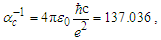
1.1. Theoretical Landscape
The first observations regarding a formalism of physically significant units were published by George Stoney in 1881 with respect to experiments concerning electric charge [12]. There did not exist a specific nomenclature with which to conveniently describe the phenomena. Thus, Stoney derived new units of length, mass, and time normalized to the existing constants G, c, and e. These units later became known as Stoney units. However, little more was discovered for the two decades that followed.In 1899, discrete phenomena became important. It was then that Max Planck submitted his paper regarding observations of quantization with respect to blackbody radiation [6]. Moreover, he resolved a new constant of nature, which he later identified as a ‘quantum of action’. Today, this is known as Planck’s constant and is denoted with the symbol h. A factor of this behavior also appeared as h/2π, later to be assigned the symbol ħ. With an understanding of c, G, and ħ, Planck was able to derive expressions for length, mass, and time with values in SI units. They are widely recognized today as Planck Units. Notably, Planck Units differ from Stoney units by a factor of α1/2 as a result of their transformation αħc↔e2/4πε0.Unfortunately, a clear physical correlation between the Planck Units and observed phenomena did not exist. Expressions using Planck Units corresponded to measurements of three digits at best. Moreover, the values for length, mass, and time were too small (e.g., the Planck time) or too large (e.g., the Planck mass) to correspond to the phenomena being measured. Over time, the Planck Units were largely relegated to the status of a legitimate discipline without a known physical significance. This said, Planck Units are still taught and used in specific branches of modern theory (i.e., superstring theory and supergravity) because of their consistency regarding many phenomena.In the century since, we find ourselves still divided by the physical constants, which are so commonly used in classical mechanics and the corresponding Planck descriptions, which in rare but specific cases carry a count term thereby recognizing the countability of phenomena. The most notable and well-understood example relates to Planck’s initial observations of blackbody radiation whereby he published his expression for energy, E=nhv, n representing the count term for Planck’s ‘quantum of action’ [6].To break the deadlock, we skip forward to the present and ask an interesting but seemingly straight-forward question. Is it the phenomenon or the measure of the phenomenon that is quantized?The question is interesting as the phenomenon of quantization has always been regarded as quantum both physically and in measure. To explore this further, we consider that we have discovered a box of pencils. First, we ask how we know they are pencils? The only answer to this is that there exists a reference pencil against which we have identified the phenomenon of a pencil and labelled it as such. We recognize that pencils are physically divisible, but for this thought experiment, we also recognize that the measure of a pencil is bounded and as such indivisible.To test our conjecture, we take the pencils from the box and place them on the desk. Our objective is to measure the phenomenon that is “pencil”. Having completed this measure, we divide the pencils into two equal stacks and measure again. Unfortunately, we are unable to evenly divide the stack. We theorize that one stack has an even count of pencils and the other odd. To test the conjecture, we proceed to divide each stack again. The process is a success with an even count stack but cannot be achieved with an odd count stack. The experiment may be repeated with the same result; the odd count stack cannot be divided. Why, because there exists no definition for half a reference and this is the physical significance of a quantized phenomenon.We could look at other means of measure and perhaps achieve some form of a division with respect to a different dimension, but if our definition of ‘pencil’ is indeed natural, that being the most fundamental of measures, then it is not possible to measure a fractional count of the reference phenomenon. Consistently, we find our efforts foiled such that the measure of the last pencil ends up in one stack or the other.There does exist one remaining concern. Thus far, we present only the notion that we cannot measure a target smaller than a natural unit. Nevertheless, can a target be smaller than a natural unit? Particles are in fact smaller than the Planck mass. Indeed, we may certainly describe a length smaller than the Planck length. Therefore, we ask the reader to entertain the idea that what exists and what is measured are physically different and that difference describes a physically important property of nature.This property will be resolved in its entirety but doing so requires a careful presentation of physical clues, one built upon the next. With that in mind, we begin Section 2.
2. Methods
2.1. Considerations for a New Approach
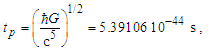
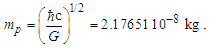
Before we express the physical constants, we must resolve values for the fundamental measures. Historically, these have been described using Planck expressions [6]. For evaluations, we used the 2010 CODATA for comparison of most calculations [2]. Once we have resolved the properties of measure, it will be better understood why the 2010 methods used to resolve Planck Units are physically more significant. Planck’s expressions [2] are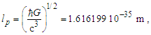 | (1) |
 | (2) |
 | (3) |
While the expressions serve as a reasonably accurate guide, they will not suffice for our purposes. For instance, if we present the expression for Planck time such that the remaining values are supplied using the 2010 CODATA, we resolve a value for G such that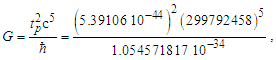 | (4) |
 | (5) |
Similarly, with respect to length, then G=lp2c3/ħ=6.67385×10−11 m3kg−1s−2 and with respect to mass G=ħc/mp2=6.67431×10−11 m3kg−1s−2. All three values disagree with the 2010 CODATA value for G=6.67408×10⁻¹¹ m3 kg−1 s−2. Is this a misunderstood geometry, new physics, or inaccuracies in measurement precision? Perhaps, but also consider that ((6.67431+6.67385)/2 = 6.67408)×10−11 m3 kg−1 s−2. Considering a 6σ correlation, geometry invites further consideration.A second and equally important issue relates to the existing classical nomenclature with which we describe nature (i.e., length, mass, time, energy, charge). Modern nomenclature does not easily accommodate descriptions of discrete phenomena. Yes, there exists a means with which to resolve or at least conjecture discrete values associated with a phenomenon, but a nomenclature that includes an independent set of discrete terms separate from the reference measures may be more successful.To succeed in this endeavor requires new tools with which to describe measure. In addition to resolving an understanding of the measurement discrepancy presented above, we need an expression that correlates the three measures—lf, mf and tf—without inclusion of the physical constants. We must identify the properties of measure. Moreover, we must understand why those properties exist and under what circumstances they are immutable or skewed.Note that working with dimensionless count terms also carries limitations [13,14] or at least physically significant rules of use. Specifically, they present an inability to:• resolve a physical quantity if there are more than three dependent variables,• derive a logarithmic or exponential relation,• resolve whether a term involves derivatives,• distinguish a scalar from a vector, and• verify dimensions given two or more dimensionless terms.The first three are restrictions on use, but in no way lessen the physical significance of MQ descriptions. Yes, use of the dimensionally correlated count terms of MQ are restricted to basic operations: addition, subtraction, multiplication and division. Nonetheless, this is rarely an issue with respect to describing most classical phenomena.The latter two limitations are cause for concern especially when working with dimensionless values such as the fine structure constant. Fortunately, the count terms used in MQ differ from the traditional definition of a dimensionless value; each count is dimensionally bound to a measure: nL to length, nM to mass and nT to time. Moreover, unlike a dimensionless value, MQ count terms may not be combined (i.e., nLnM≠n2). Finally, each count term is, in definition, correlated to its dimensional counterpart: l=nLlf, m=nMmf, and t=nTtf. While attention must be given to avoid expressions that are dimensionally ambiguous, rarely do the issues typical of dimensionless values become physically significant in MQ.
2.2. Physical Significance of Measure
Before we begin, we must distinguish the fundamental measures of MQ from those of Planck. A subscript p is used to specify Planck units, whereas a subscript f is used for the fundamental measures, specifically, lf for length, mf for mass and tf for time. In that we have not resolved the fundamental measures, we use Planck Units as a guide. The arguments and expressions are to be considered as such until the properties of measure and the values of the fundamental measures are resolved.Beginning with our understanding of light and Heisenberg’s expression for uncertainty [15,16], we resolve both counts and values for each measure. The speed of light is described as a count nL of length units lp divided by a count nT of time units tp, then c=nLlp/nTtp such that | (6) |
Using c=lp/tp and Planck’s expressions for length and mass, we also resolve that the product of their squares is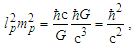 | (7) |
 | (8) |
Finally, using Heisenberg’s expression [16] to describe the uncertainty associated with the position σX and momentum σP of a particle, | (9) |
we can resolve physically significant values for nL, nM, and nT. We begin by clarifying how we intend to use Heisenberg’s expression to achieve our goal. This involves identifying the physical properties of uncertainty we intend to isolate.The uncertainty principle asserts a limit to the precision with which certain canonically conjugate pairs of particle properties can be known. However, this differs from our goal of resolving the certain minimum measurements of a particle at the threshold, ħ/2. Therefore, we introduce a special case of the use of variances.Although the expression for variance is usually written to describe the certain properties of many targets, we modify this usage to describe the certain properties of many measurements whereby the measurement, whether applicable or physically significant, is uncertain. With this, we then consider the solution for only the minimum count values for length, mass, and time such that the conjugate pair is equal to the threshold at ħ/2; that is,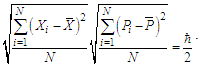 | (10) |
To the extent that the minimal count N is reducible to a certain measure describing a single particle, we consider measures at N=1. The variance terms for position and momentum reduce such that there is a certain length 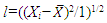 corresponding to the variance in X and a certain momentum
 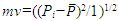 corresponding to the variance in P. We write each term in the MQ nomenclature, i.e., l=nLrlp and mv=ml/t=nMmp(nLlp/nTtp). Note also that the count nL for the change in velocity is distinct from the position count nLr, the latter describing the distance between the observer and the particle. We have
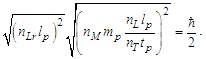 | (11) |
With these constraints, it follows that the minimum count values at the threshold ħ/2 correspond to a minimum distance nLrlp and a momentum comprising a minimum mass nMmp, a minimum length nLlp and a minimum time nTtp. Replacing the value of ħ with the result from Eq. (8), we then have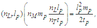 | (12) |
 | (13) |
Identifying two additional conditions, we may constrain the expression sufficiently to resolve the count values for each dimension. We begin with a description of G using the expression for escape velocity.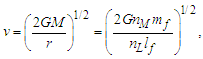 | (14) |
Such that v=nLlf/nTtf, given that nL=nT=1 (Eq. 6) and nM=1/2 (Eq. B7), we resolve that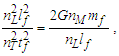 | (15) |
 | (16) |
To resolve the second condition, we return to the expression for escape velocity, again reducing the expression to Planck units and/or counts of those units. Such that r=nLrlp and M=nMmp and where we consider G at the bound v=c, then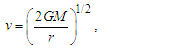 | (17) |
 | (18) |
 | (19) |
Given 2nLrnMnL=nT (Eq. 13) and nL=nT (Eq. 6), then | (20) |
Then, as expected, with nLr=2nM (Eq. 19), we find | (21) |
 | (22) |
 | (23) |
We may continue the reduction given nL=nT (Eq. 6) and 2nLrnMnL=nT (Eq. 13), whence we obtain | (24) |
 | (25) |
Along with nL=nT (Eq. 6) and such that nL and nLr describe the phenomenon of length, then | (26) |
Thus, we recognize with the observation thatO1: There are physically significant fundamental units of measure: length, mass, and time.That is, there is a physically significant lower threshold to measure as described by the resolved counts. The measures do not imply that a phenomenon may not be less than a minimum. Rather, a length or elapsed time less than lp and tp may not be measured with greater precision. Notably, mp is a composite of the length and time, an important count but not a minimum measure. Moreover, the above calculations do not imply that measure is discrete or countable. Resolving these properties requires further analysis.
2.3. Discreteness of Measure
We now entertain measures larger than the bounds identified in the prior section. Again, as before, we describe measure as a count of some fundamental unit of measure, in this case, a count of the fundamental unit of length. We also expand our analysis to include macroscopic measures (i.e., any distance greater than the reference lp). By example, consider two sticks, one a length of 5.00 lp and the other a length of 5.25 lp. The difference may then be described as | (27) |
Is the result measurable? No. As resolved above, any count of the fundamental measure less than 1 cannot be measured. Therefore, with respect to the Heisenberg uncertainty principle, the gravitational constant, the speed of light, and the expression for the escape velocity, this difference cannot be measured. This is also to say that all macroscopic measures may be observed only as a whole unit count of the reference measure.While the presentation is extendable, let us clarify with another length difference, two sticks such that one is 10.25 lp and the other is 5.00 lp, | (28) |
The difference here is physically significant and not discrete. To verify this statement though would also require that the result be distinguishable from a whole unit count equal to five units of the reference. We compare the result with a count of 5 lp, | (29) |
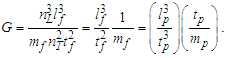
We find again that this case is the same as the first. Thus, we can conclude that measure is physically significant only if a whole unit count of the reference is made. This may be summarized with the following observations:O2: Fundamental measures are discrete and countable.O3: Fundamental measures length and time each define a reference.We single out fundamental mass as exempt from this analysis. Mass is a consequence of our description of length and time. It is not a physically significant minimum measure. By example, one may resolve an expression for length starting with the expression for time. This arises in all physical descriptions of either dimension by definition of their measure (i.e., divide lp by c to get tp). Conversely, one may not resolve a value for length or time starting with the expression for mass. The realization that G=lf3/tf2mf is a consequence of the observation that the measure of G is coincident with this relation. To use that realization to establish physical significance is circular.
2.4. Measurement Frameworks
As established to this point, we recognize that measure is a property of references. With respect to this observation, we can then consider that the universe may be described as a space, time and mass. Locations in that space represent places of observing mass in elapsed time. And with respect to every place the visible motion may not exceed c. In that the rate of visible motion from all places is defined by the maximum c, we also recognize that the classical definition of a universe as a physically significant frame can have no external reference. Importantly, we then observe that measure with respect to the universe (i.e. with respect to the space) must be non-discrete.The observation brings to our attention a big picture view of measure, non-discrete with respect to the universe yet discrete relatively between objects. It is for this reason we describe measure with respect to the universe using a self-defining frame of reference. We describe measure relatively between phenomena using a self-referencing frame of reference. Distinguishing the properties of measure and how we describe measure enables a clearer description of phenomena.In working through various examples, we demonstrate that it is the difference between these two frames of reference that give rise to many, if not all, of the constants and laws of nature. If it were possible to reference points external to the universe, there would exist no differential between two frameworks and many of the observed behaviors of nature would not exist. With these observations, we observe thatO4: Measure with respect to the observer is discrete.O5: Measure with respect to the universe is non-discrete.To demonstrate these observations with a mathematical description applicable to an observable phenomenon, we propose an experiment that may be described by each of three frameworks. A frame describing measure with respect to the universe carries the property of non-discreteness. The remaining two carry the property of discreteness. The experiment also abides by two design prerequisites. We introduce no additional measures, such as angles, and at every instant in time, the observer must have access to all available information.Using the standard understanding of a Cartesian coordinate system, we illustrate the three frameworks in Fig. 1. With respect to the different origins of information (i.e., the frameworks), we then recognize the differences in the discreteness of measure. The three frameworks are:• Reference Framework—This is the framework of the observer where properties of the reference  are observed. With respect to the standard understanding, this framework differs only in that measure is a count function of discrete length measures equal to one.• Measurement Framework—This framework shares properties with the Reference Framework. It is characterized as some known count of the reference describing where count properties of the reference
  are observed.• Target Framework—This framework is characterized by the property of measure of non-discreteness, that being the framework of the universe that contains the phenomenon
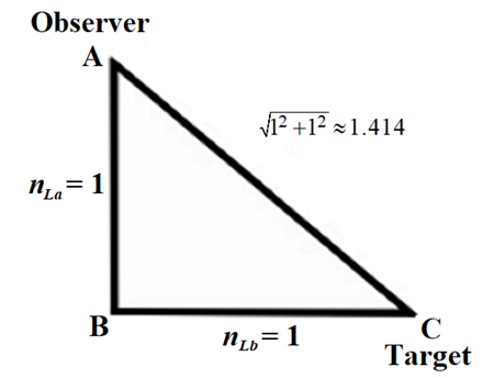 | Figure 1. Count of distance measures along segment  |
Although each framework is described with respect to the observer’s point-of-view, we also recognize the different properties of measure associated with each framework. With these constraints, we now address how information regarding the count of length measures in the Measurement Framework is obtained by the observer relative to the Reference Framework. Moreover, we make this presentation to establish values for the fundamental measures. As such, we will no longer use Planck Units, instead proceeding with the terms lf, mf and tf. Consider a system of grid points separated with a fixed count of lf along the shortest axis. Specifically, there must be enough points to form a square such that the length of each hypotenuse of the square is also equal. To set up the grid initially, we propose that a laser pulse rangefinder is used at each point along with the time-of-flight principle to ascertain a match to the prescribed requirements. In this way, we ascertain that the angular measure at each point is either along a line or at 90° except for those points along a hypotenuse. The design, as such, does not require that we introduce angular measure. Moreover, as all prerequisites are agreed prior to setup, the experiment does not initially incorporate time.Note that there are two discrete frameworks, one in which A certifies the length  (the Reference Framework) and the other in which C certifies the length
  (the Measurement Framework). The Target Framework contains both A and C for which the unknown length
  is a member. In this way, all information in the system is defined with only the presence of members A and C.Using the Pythagorean Theorem such that
  we recognize that
  However, with respect to the observer only a discrete reference count may be measured of
  It is with this conflict that we conclude that the difference 1.414−1.000=0.414 describes a physically significant property of the universe. In the section that follows, we show that this difference is the phenomenon of gravity.
2.5. Gravity
Having resolved that measure has a lower threshold and is discrete and countable, we now address the physical significance of a phenomenon with respect to the discrete and non-discrete frames. The three frameworks described in Section 2 are represented in Fig. 2. Side a is always the reference count 1. Side b is some known count of the reference. The hypothenuse of the right-angle triangle Side c is then resolved using the Pythagorean Theorem.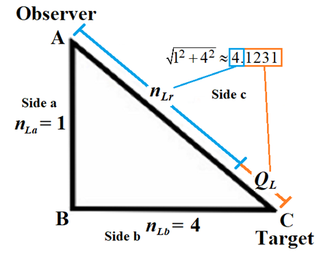 | Figure 2. Count of distance measures between an observer and target |
Importantly, as a reference, Side a is prerequisite to any count of the reference along Side b to resolve Side c. Assigning a count other than 1 to the reference would introduce a factor representation (i.e., a=2) of the reference for all sides concealing the discrete count properties of the described phenomenon. Hence, | (30) |
We conjecture that any non-integer count QL of the reference along the unknown Side c relates to a change in distance. We may describe this as repulsion when rounding up or attraction when rounding down. Notably, for all solutions, QL is less than half as evident by its largest value ~0.414 at Sides a=b=1 and therefore attractive. Moreover, because Side c always rounds down, we find that nLr=nLb for all observations. Thus, for each count nT of fundamental time tf, the model describes a count of lf that is closer by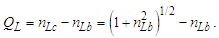 | (31) |
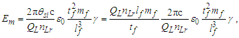
Because the measure of Side c always rounds down, moving forward, we replace the term nLb with nLr. We also identify nLr as the ‘observed measure count’. With the loss of the remainder QL relative to the whole unit count is QL/nLr, we now have an important dimensionless ratio that describes gravity.We may express this ratio in meters per second squared (m s−2) by multiplying by lf for meters and dividing by tf2 for seconds squared. This describes the loss of distance at the maximum rate of one sampling every tf seconds per second, | (32) |
When compared with a classical description, we notice now that the quantity is scaled. Hence, we introduce the scaling constant S, multiplying by c/S to resolve. Notably, c describes the rate of increasing space relative to observers in all spaces as identified with respect to the classical description of the universe. In the following, we will learn that the scaling constant S is fundamental to the relation that describes the three measures. Such that r=nLrlf and c=lf/tf, then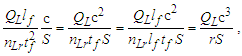 | (33) |
 | (34) |
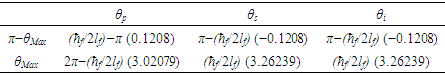
The expression describes gravity as the difference between the non-discrete measure with respect to the universe and the discrete measure of the observer. When compared with Newton’s expression G/r2, we see a distance between the two curves that is immeasurable, beyond the sixth digit of precision for all distances greater than 2,247 lf. The curves differ by QLnLr, which describes a skewing of measure due to the discreteness of measure, an effect we refer to as the Informativity differential. As derived in Appendix A, QLnLr approaches 1/2 with increasing distance.In Appendix B, we replace S with θsi because of its correlation in value to the signal and idler polarization angle with respect to the plane of X-rays at maximum quantum entanglement [3]. Notably, the term is not a radian for all contexts, but the value of θsi=3.26239 is constant for all physical contexts. For instance, when the expression for mass accretion is written such that Macr=θsi3mf/2tf ([7], Eqs. 135 and 136) then θsi is dimensionless, having no units at all (note: Macr is a rate kg s−1). Likewise, as expressed in the fundamental expression lfmf=2θsitf ([7], Eq. 47), θsi has units kg m s−1. As demonstrated in Eq. (B7), θsi has units of radians. Each measure of θsi is physically significant and corresponds to the measurement data to six significant digits.So, why does this constant differ from the other constants that we are so familiar with? In part, because the other constants are each a composite of this constant and in part because this constant is a composite of all three dimensions θsi=lfmf/2tf. The units carried by θsi depend on the phenomenon and the selected frame. Described with respect to the Measurement Frame, θsi usually carries the units of momentum. Described with respect to the Target Frame of the universe, θsi carries no units. For specific descriptions with respect to electromagnetic phenomena, θsi carries the units of radians. Examples are presented throughout the paper, but for nearly all cases, θsi is defined with respect to either the Measurement (kg m s−1) or the Target (dimensionless) frame.
2.6. Fundamental Measures
With a quantum definition for gravity, we can now resolve the simplest relation that describes the fundamental measures. This approach is sensitive to the skewing effects of discrete measure and as such we cannot use the measure of ħ, a quantum property resolved where the effects described by the Informativity differential (Appendix A) are significant. Conversely, use of the measures of c and G are acceptable. Note also that the units for θsi are kilogram meters per second. As described in Appendix C, we then have: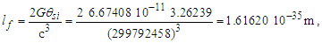 | (35) |
 | (36) |
 | (37) |
We may approach a solution to the fundamental expression—the simplest expression that relates the three measures—in two ways. One is we may replace G given that G=c3tf/mf (Eq. 16); the other is we may solve for G using the expressions for lf and mf, then set them equal and reduce. That is, | (38) |
 | (39) |
Here, all counts in Eq. (38) are notably equal to a value of one. This differs from their minimum values as well as the count for mass, nM=1/2 (Eq. 23). Explicitly, the fundamental expression is not a description of the lower count bound of each dimension. Moreover, in MQ, we often ignore the Informativity differential and instead replace QLnLr with its macroscopic limit of ½ as described in Appendix A. The more precise expression, which we refer to as the expanded form, is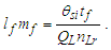 | (40) |
As such, many MQ expressions are affected by the Informativity differential, each having expanded counterparts. Although the calculation does involve several steps, it is required when describing quantum phenomena, especially phenomena less than 2,247lf.
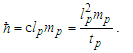
2.7. Physically Significant Discrepancies with ħ
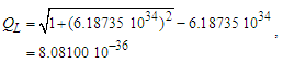
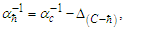
Expressions that use measures, both macroscopic and quantum, have limited precision because of the Informativity differential. In this section, we explore those effects as they apply to the measures of G and ħ. This was demonstrated in (Eqs. 4 and 5) where the resolution of the gravitational constant using Planck’s expression for time presented a discrepancy in the fourth significant digit, a value of 2.4×10⁻¹⁵ with respect to the 2010 CODATA. Because the measure of G is a property of macroscopic phenomena and ħ a measure of quantum phenomena, it is necessary to resolve the effects of the Informativity differential to present a value of ħ as it would appear if measured macroscopically. We will call this ħf. This, in turn, would be suitable when measured in expressions that include measures resolved macroscopically.Given c3/G=ħ/lf2 (Eq. 1) and the fundamental expression θsi=lfmf/2tf (Eq. 39), we resolve ħf with respect to macroscopic measures G=c3(tf/mf) (Eq. 16), then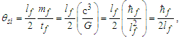 | (41) |
 | (42) |
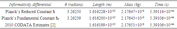
The approach physically validates our understanding of the derivation of limnLr→∞f(QLnLr)=1/2 (Appendix A), which had we instead used the expanded form of the Informativity differential (Eq. 38), would then yield ħ=θsilf/QLnLr. The result describes Planck’s reduced constant at the macroscopic limit, although the measure of ħf at any distance greater than 2,247lf will reasonably approximate the limit.Conversely, at the quantum distance 84.9764lf (Appendix D)—that distance corresponding to the measure of blackbody radiation—and ħ=θsilf/QLnLr with QLnLr = 0.499983, then the value of ħ is as we recognize it today. We identify the 84.9764lf distance as the blackbody demarcation.Note that ħf is a function of only θsi and lf when accounting for the contraction of length associated with discrete measure. The approach changes our understanding of the physical significance of ħ, now being a count property of the Heisenberg uncertainty principle. Importantly, the Planck discrepancies observed in Eqs. (1)–(3) with respect to the 2010 CODATA are reduced to the sixth significant digit (see Table 2).Table 2. Planck’s expression calculated with quantum ħ and macroscopic ħf values for Planck’s constant
 |
| |
|
We mention that the small rounding effect that occurs in the length result (0.0000006×10⁻³⁵ m) is subsequently amplified in the mass. Had the rounding gone the other way, differences with the CODATA would not exist. That said, neither case displays a seventh-digit physical significance and as such should not be considered. There exists no physically significant difference between the MQ description and the measurement data.With Planck’s reduced constant adjusted for the effects of the Informativity differential, we may apply the value to expressions that include macroscopically measured terms. For instance, the value of θsi as described in Appendix B using G and c may now be presented using ħf (see listing in Table 3). Each value precisely matches the Shwartz and Harris measures [3].Table 3. Predicted radian measures of the k vectors of the pump, signal, and idler for the maximally entangled state at the degenerate frequency of X-rays using Planck’s fundamental constant ħf
 |
| |
|
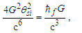
Likewise, we may expand our understanding of the relationship between G and ħ with the following correlation. We start with the fundamental expression lfmf=2θsitf (Eq. 39), then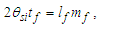 | (43) |
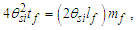 | (44) |
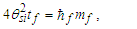 | (45) |
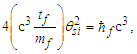 | (46) |
 | (47) |
Here, all the terms are macroscopic, and hence we have appropriately replaced ħ with ħf. We then move the terms we find in Planck’s expression for length (Eq. 1) to the right, leaving the remaining terms for the fundamental length (Eq. 35) to appear on the left. This brings to our attention that it is the lack of the Informativity differential that limits Planck’s expressions to three digits of precision. Having both a physically significant description of the fundamental length and accounting for the skewing effects arising from discrete measure, we bring the two expressions together thus resolving the measurement discrepancy found in G as presented in Eqs. (4) and (5). Specifically, we have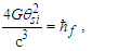 | (48) |
 | (49) |
 | (50) |
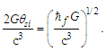
In the same way, we can take this expression and using ħf, Planck’s reduced constant adjusted for the Informativity differential, solve. However, (ħG/c3)1/2=1.61623×10−35 m incorrectly resolves the measured value. Using ħf, the expression is now mathematically equivalent to six digits,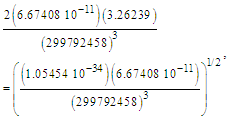 | (51) |
 | (52) |
Returning to Eqs. (4) and (5), and replacing ħ with the distance sensitive measure adjusted for the Informativity differential, ħf, the discrepancy with the 2010 CODATA for the gravitational constant G=c3lp2/ħ=6.67385×10−11 is also resolved, specifically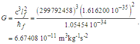 | (53) |
Moreover, replacing ħ with ħf properly accounts for the skewing effects of the discrete measure as applies to Swartz and Harris’s measure of θsi (Appendix B),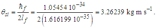 | (54) |
The dimensional homogeneity problem is also solved. From the fundamental expression, 2θsi=lfmf/tf, we find a mathematical correspondence with the 2010 CODATA values [2],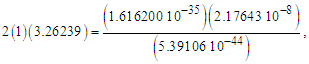 | (55) |
 | (56) |
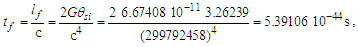
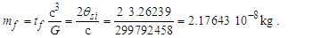
Finally, we recognize that the quantum approach to describing gravity also allows for a calculation of the gravitational constant using only the measure of light (i.e., lf =tfc) and θsi. The approach again corresponds to the 2010 CODATA to six significant digits.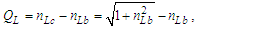 | (57) |
 | (58) |
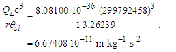 | (59) |
Similar examples extend to electromagnetic phenomena. The effects of the Informativity differential with respect to those constants will be discussed in the section to follow. To summarize these results, we present in Table 4 the Informativity differential with respect to three physical constants. We recall that the value for θsi comes from the Shwartz and Harris experiments, not from the CODATA, which presently does not recognize this value.Table 4. Physical constants calculated with quantum ħ and macroscopic ħf values for Planck’s constant
 |
| |
|
3. Results
3.1. Fine Structure Constant
Considering the new descriptions offered by MQ, we present four expressions that describe the fine structure constant α. Concepts from MQ are used to resolve an understanding of each. More importantly, we present a singular physical description of their differences— that is, how the distortion of measure explains the difference in value between each expression.Before we begin, we note that counts of θsi are central to the presentation. Specifically, the count factor 42 of θsi determines the value of the fundamental fine structure constant αf and is physically correlated to the charge coupling demarcation, a distance associated with α and described as a count of lf. The two terms—lf and θsi—are proportional as described by the count values of each term and related by the fundamental expression. Given the minimum count terms are nL=nT=1 and the corresponding count term for mass nM=1/2, (Eqs. 23, 26), then the minimum count of θsi with respect to the Reference Frame is obtained from the fundamental expression, | (60) |
The physical significance of counts and their relation to frames of reference are best understood with respect to the unity expression described in ([8], Eq. 111) of a “Quantum Model of Gravity Unifies Relativistic Effects …” as published in Journal of High Energy Physics, Gravitation and Cosmology; | (61) |
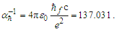
As is true with the fundamental expression, the combination of terms lfmf/tf has no units, defined with respect to the frame of the universe. The unity expression describes the dimensional measures of the prior counts with respect to the expansion of the universe, yet notably excludes the factor 1/2, the constant of proportionality in the fundamental expression lfmf/2=θsitf which correlates the dimensional terms. When working with the nondimensional expressions of MQ, how counts apply to specific phenomena must be validated by the physical and value correlations of the resulting description, the difference in this case being a description with respect to the self-defining frame of the universe, as opposed to the self-referencing frame of the observer.With respect to the charge coupling demarcation a non-discrete distance of nLr=276/θsi=84.6005 corresponds to a count of nθ=RND(84.9764/2)=42 in the Measurement Frame. We present the MQ expression for the inverse of the fundamental fine structure constant as αf−1=42θsi. However, θsi is defined with respect to the Target Frame and as such is dimensionless. A second description of α was discovered by Planck in his work with the Planck units. He observed that α could be described as a function of the electron mass me and the radial distance to the first ground state orbit a0 (i.e., the Bohr radius 4πɛ0ħ2/mec2). We identify his description with the designation αp. A third description follows from electromagnetism, which also serves as the CODATA definition for α. We identify this description as αc. A fourth expression follows from MQ, modifies the CODATA definition such that Planck’s reduced constant ħ is adjusted for the Informativity differential, ħf with respect to a macroscopic distance. We identify this description as αħ. There are other descriptions, such as α=Z0G0/4 written as the impedance and conductance of a free vacuum and the product of the Bohr radius α=re/rQ such that rQ=ħ/mec. The first four descriptions though will suffice for our demonstration.We shall next discuss the metric and Informativity differentials and their relation to each of the measurement frameworks. We do not address the change in the value of α with respect to increasing energy as described in QED. Nonetheless, this presentation does address the ground state of α; a description that incorporates high-energy phenomena is to be a topic of further research. Also, we note that αħ is not physically interesting because a coupling of the Informativity differential to the measure of a phenomenon that already accommodates the effects of this skew is duplicative. Given that ħf differs from ħ precisely by the Informativity differential, the calculation presents an opportunity to demonstrate two means of applying this effect, each resulting in the same value. The expression and value for each of the four descriptions are: | (62) |
 | (63) |
 | (64) |
 | (65) |
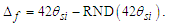
To explain their relationship, we begin with αf and then demonstrate how each of the remaining expressions differ. Two distinct measurement-skewing effects must be considered. The metric differential is notably different than that of the Informativity differential; the latter describes the skew in measure arising from the discreteness of measure and is defined with respect to the self-referencing frame of the observer, that is, between phenomena in the universe. The metric differential Δf describes the shift in measure that exists between the discrete and non-discrete frames. The function RND to be used below means to round to the nearest whole-unit value (glossary). And the count nθ is 42, as discussed above, corresponding to the measure of the charge coupling demarcation.Beginning with a general expression for the metric differential, then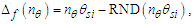 | (66) |
 | (67) |
To resolve a Planck form of the expression αp−1, we start with αf−1 and adjust; that is, we add the metric differential Δf. The addition accounts for the physically significant difference between the discrete and non-discrete frames of reference.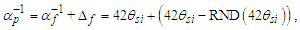 | (68) |
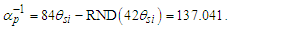 | (69) |
The value is identical to the value resolved with Planck’s expression to the precision of θsi, i.e., six digits.Conversely, descriptions of αc and αħ differ from that of αp by the Informativity differential. To proceed, we must know the non-discrete count nLr of lf associated with the charge coupling of a cesium atom absorbing a photon, namely, the charge coupling demarcation, described here;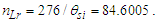 | (70) |
We can then resolve the Informativity differential as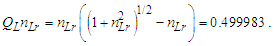 | (71) |
The differential skewing of measure between the Planck and electromagnetic expressions Δ(P-C) due to MQ is again the differential between αp−1 and αc−1. We multiply the Informativity differential by two to resolve the skew with respect to the self-defining frame of the universe, not the radial description respective of an observer/target relation. Then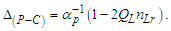 | (72) |
Notably, the Informativity differential is a contraction effect (i.e., like gravity). Subtracting two differentials 2QLnLr of αp−1 from αp−1 (i.e., 1−2QLnLr), then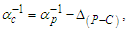 | (73) |
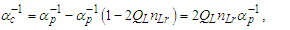 | (74) |
 | (75) |
We repeat this process once again to resolve the value one would find when using the Informativity differential adjusted value for Planck’s constant, ħf, only our base measure is not αp−1, but now αc−1. Specifically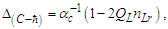 | (76) |
 | (77) |
 | (78) |
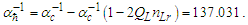
Each of the values match the corresponding 2018 CODATA values to the same precision as the measure of θsi, i.e., six digits. Also, of interest is the difference between the calculated values with respect to the modern and MQ expressions. While MQ calculations are constrained to six digits of physical significance —the precision with which we can measure θsi—on comparing the values of the resulting calculations, we find that the difference between the modern and MQ expressions are consistent to the 10th significant digit corresponding to the precision of the modern measurement (see Table 5). The consistency of the difference emphasizes a correlation that extends in parallel between the MQ expressions and the physical measurements.Table 5. Modern and MQ expressions for the inverse fine structure constant, their values and difference
 |
| |
|
Moreover, we now have one physical approach to describe all expressions. The difference between them is a function of the differential. The approach supports the position that the expressions are not in error but are a physically significant consequence of MQ relative to the measurement distance. This is most relevant in the long-standing discrepancy between the Planck and electromagnetic interpretations. There has been no physically correlated explanation for their difference to date. We also draw attention to the metric differential and its physical significance when describing differences in measure between the two frames of reference.
3.2. Electromagnetic Constants
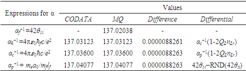
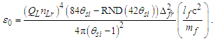
Until May 20, 2019, the value of the elementary charge e had been defined as an exact number of Coulombs [17]. This gave a specific value for the electric constant ɛ0 as a function of the magnetic constant μ0, which in turn follows from the elementary charge and the fine structure constant α. This approach has changed. Now, the elementary charge, Planck’s constant h, and the speed of light in vacuum c are defined values, leaving the magnetic constant as a measured value that determines the value of ɛ0. The magnetic constant, as before, is a function of α.With the expressions presented, we may approach definitions for the electromagnetic constants anew. For one, we may replace Planck’s reduced constant with the following expression (Eq. 54) given QLnLr=1/2, | (79) |
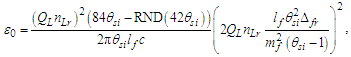
Next, we may replace α with αc reducing the description of ɛ0 to a function of θsi, c, and e. Although ɛ0 is defined, the determination of ɛ0 follows as a function of e, fundamental units, and mathematical constants. With QLnLr=0.499983 at the charge coupling demarcation, then | (80) |
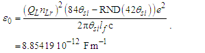 | (81) |
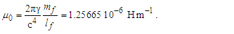
Given that μ0=1/ɛ0c2 and c=lf/tf, we also resolve two more constants. The magnetic constant, for instance, is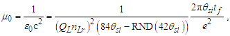 | (82) |
 | (83) |
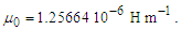
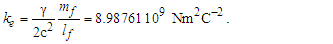
Coulomb’s constant ke is | (84) |
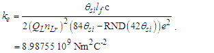 | (85) |
New to modern theory, θsi is also the radial rate of expansion defined with respect to the universe (i.e., not per Mpc) and an angular measure (in value) corresponding to the plane of polarization for maximally quantum-entangled X-rays in specific Bell states [3]. As such, we have expanded our physical definition of electromagnetic theory to include both quantum and cosmological phenomena.Although the electric and magnetic constants have been reduced, in part, as a function of the metric and Informativity differential, elementary charge remains problematic in that a known description of e does not exist as a count of θsi. That is, the non-discrete frame of the universe provides a geometry of only counts and mathematical constants. Nevertheless, elementary charge is a multi-dimensional measure in the discrete frame of the observer. For this reason, there exists no mathematical counterpart. We are forced to describe e with a discrete physical approach and correlate that to the non-discrete frame of the universe with the metric differential.Before we begin, we note briefly that a second way to describe the metric differential is as a ratio of counts of θsi. Specifically, we introduce the quantization ratio, taking the non-discrete product nθθsi and dividing by its discrete product,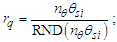 | (86) |
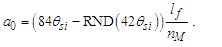
Its physical significance is discussed extensively in the sections to follow. We may now resolve an expression for elementary charge. Recall in Eq. (69), that αp−1 was resolved with respect to a differential (i.e., a difference) between the discrete and non-discrete frames, i.e., 42θsi-RND(42θsi). As such, we may describe the differential b-d of ef as an equality with the quantization ratio b/d. Collectively, the two define the fundamental elementary charge which when multiplied by the metric differential Δfr between the frames – the product being a function of rq and b-d (i.e., b/d=b-d) – give us ep in the local frame. To do so, we leverage the known value of the discrete difference d=θsi at the demarcation 42θsi. Notably, the demarcation counts for all phenomena round to 42. | (87) |
With this we isolate and resolve the fundamental value of ef as a function of b. Keep in mind, charge is not and may not be known as a count of θsi nor is it known in terms of the fundamental measures. As such, there exist no dimensionally homogeneous precedent to validate our expression. To compensate, we express all measures in their fundamental form, lf, mf, tf, θsi, and ħ, replacing dimensional homogeneity with physical homogeneity.Having physically correlated each measure, then the base b is the elementary charge ef as a function of the fundamental mass f(mf) relative to its quantum of angular momentum ħf. We begin by mapping each description to θsi. For instance, the corresponding momentum is θsi=(1/2)lfmf/tf, indicating that we should divide ħf /2. Moreover, we observe that the phenomenon of elementary charge presents itself at the upper bound c. Therefore, we resolve the upper count bound of mf in relation to the count of tf as the mass frequency bound. As described in Appendix E and the third paper ([9], Appendix 5.3), then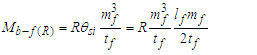 | (88) |
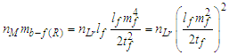 | (89) |
Hence, f(mf)=mf2 relative to θsi=lfmf/2tf (i.e., the remaining terms). With both mapped to θsi, then the physically homogenous expression is b=mf2/(ħf/2). With this description resolved with respect to the macroscopic measures of G and c, we then use ħf=2θsilf to reduce. Thus, | (90) |
The approach confirms the identification of θsi as the divisor/difference d. We remove θsi from our definition of the base b and account for the squared relation of mf at the bound, | (91) |
We now solve for the fundamental elementary charge in terms of the fundamental units, | (92) |
 | (93) |
 | (94) |
With respect to units, there is no convention in describing phenomena relative to different frames. The issue becomes more complex with elementary charge, now a presentation of the geometry used to describe the fundamental fine structure constant. It is conjectured that charge may have a geometric origin, a function of m kg-2, but more research would be needed to fully resolve the physical significance of this description.We continue by correlating this description to the Measurement Frame by applying the metric differential. This is described as a product of the quantization ratio between the two frames. Note, the differential is an offset of one relative to the demarcation. The differential should have been applied to ef, but we are forced to apply it to ep, making this an approximation. That said, a solution is presented in Section 3.7 that resolves the true value. For now, we describe this as nθ-1 such that nθ=42.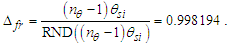 | (95) |
Taking the product, we resolve the Planck equivalent of elementary charge.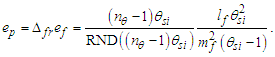 | (96) |
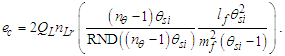
We present the Informativity differential relative to the demarcation count (both the charge coupling and blackbody demarcations product the same six-digit value) and resolve the differential between the Planck equivalent ep and the CODATA form of the elementary charge ec;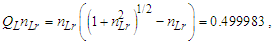 | (97) |
 | (98) |
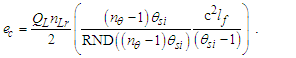
Subtracting two differentials 2QLnLr of ep from ep (i.e., 1-2QLnLr), then | (99) |
 | (100) |
 | (101) |
 | (102) |
With a description of the elementary charge comprising fundamental measures, we describe the electric and magnetic constants. Such that lfmf=2θsitf and ec=2QLnLrep=2QLnLrΔfref, then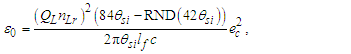 | (103) |
 | (104) |
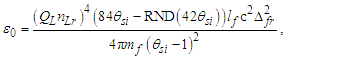 | (105) |
To be discussed in detail in the section on unification, we may replace the metric differentials with gamma γ. The effects described by γ are geometric, a function of the point-of-view of the observer and not intrinsic to the described phenomenon. For this reason, it is physically significant to separate these characteristics.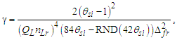 | (106) |
Making the substitution then,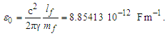 | (107) |
With μ0=1/ɛ0c2, then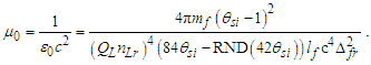 | (108) |
 | (109) |
Coulomb’s constant is then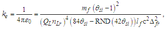 | (110) |
 | (111) |
The value of each constant is compared with the 2018 CODATA values in Table 6.Table 6. Electromagnetic constants as a function of the fundamental measures and appoximated γ
 |
| |
|
Notably, there is a skew of 0.55 in the sixth digit of e from that found in the CODATA. This stems from the application of the differential to ep instead of ef. Moreover, there is a six-digit precision constraint in the measure of θsi that is amplified in ɛ0 and ke. We will address this by resolving a more precise value for γ in Section 3.7.To explore the physical meaning of these expressions further, we modify the definition of μ0 to incorporate h as a part of the expression. First, recall that the blackbody demarcation (Appendix D) is a function of the Informativity differential, which may be used to solve for the demarcation at 84.9764lf. With this solution, we resolve first the metric differential Δfr=0.998194 and then the Informativity differential QLnLr=0.499986. Given ħf=2θsilf, then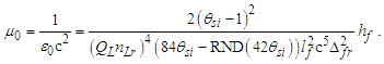 | (112) |
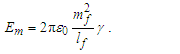
The expression hints at magnetic phenomena being a discrete count of Planck’s constant, a quantum of action. Does this tell us more about its discrete properties? Perhaps, but we must refine this understanding to improve the physical correlation. The focus here is on π, which was lost with the introduction of hf. To understand the physical importance of π, observe the expressions below; they describe the relationship between the energy of a fundamental unit of mass Em and the energy of a photon El. From the fundamental expression lfmf=2θsitf and with ħf=2θsilf (our comparison is with the measure of mass), then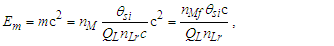 | (113) |
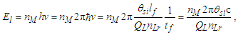 | (114) |
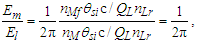 | (115) |
 | (116) |
These expressions describe the role of π between descriptions of particle and wave phenomena. That is, the numerical constant that divides them is 2π. Returning to the Planck modified definition for μ0,we find that it is more fundamental to retain π. This is evident when we observe that the difference between Eqs. (108) and (112) is | (117) |
Such that (2θsilf)=ħf, it is more fundamental to replace hf and then ħ, which would then place us back to where we started. That is, electromagnetism is best described as a wave phenomenon (epitomized by π) in a classical spacetime using the same fundamental measures used to describe gravitational curvature.That said, we also observe that | (118) |
With γ incorporating several effects, each a function relative to the observer, then the discrete properties of Planck’s constant hf, the quantum of action, are directly proportional to that of μ0.
3.3. Properties of the Atom
When working with the MQ nomenclature, we may more easily recognize the permissible properties of phenomena. For instance, we may ask what an MQ description of an elementary charge looks like to understand atomic structure. With the observation of charge appearing in nature as a discrete count of fundamental units, we may then look to the component terms to see if they vary and, if so, what other values of e are permitted. From Eq. (101) and given θsi2/mf2=c2/4, then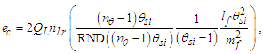 | (119) |
 | (120) |
We observe that all values are constant. Subsequently, given that elementary charge is measured only as a whole-unit count of e, we find that charge must be a whole-unit count of the observed phenomenon. Importantly, the component terms that describe e are physical and numerical constants. To imply that e could take on a fractional value would require that one or more of the fundamental measures—lf or θsi or c—was not fundamental.The description does not accommodate fractional charges inferred with respect to quarks, leaving the conjecture that charge is a physically measurable property of quarks unsupported.O6: Charge is not a physically measurable property of quarks.In a similar fashion, such that me=nMmf, (i.e., nM is not a physically significant count, but is constant) Planck’s expression for the fine structure constant may be arranged as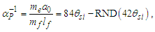 | (121) |
 | (122) |
Consequently, the ground state orbital a0 of the electron must exist precisely as described.O7: The ground state orbital of an atom is invariant with respect to the fundamental length lf and the count nM of mf of an electron (i.e., lf/nM).There are no variable terms in the description. Importantly, we find that the Informativity differential, applicable to terms in the numerator and denominator, cancels out such that it is also not a part of the description. Thus, we would expect differentials are a function of the relative distance of the observer, not an intrinsic property of the atom.
3.4. Unification
One of the greatest endeavors of the modern era has been to provide a physically significant and meaningful unification of gravity with electromagnetism. We present that this endeavor is challenging in that there is no clear roadmap as to what constitutes unification. For instance: i) Should one present a one-for-one match between strings as described in String Theory with respect to each of these phenomena? ii) Would this be recognized as the most satisfactory solution? iii) Would a correlation between two distinct field expressions constitute a better unification? iv) What about a classical approach using only the laws of motion?Moreover, let us consider the existence of a match. In that each phenomenon is different, there would exist a physical differential. What differential—additional constants and geometry—would be acceptable?Let us entertain what may be considered a step towards unification by presenting an example of what is not unification to help clarify the definition. Consider the expression for the product of the electric and magnetic constants and multiply both sides by G, | (123) |
Granted, such a coupling of fields is nonsensible, but our goal is to then reduce and demonstrate a fundamental expression that masquerades as unification. With G=c3tf/mf, replace G on the right-side, thus solving for G. | (124) |
 | (125) |
Why does this fail to demonstrate unification? Among other things, the expression fails to provide term descriptions that can be defined independent of the unified phenomena. With this example, we identify unification as beingnomenclature of physically distinct terms that are independent of the correlated terms,A definition of each correlated term comprising distinct terms and mathematical constants, andA difference between the correlated terms that describes one or more other phenomena.Consider now the application of the MQ nomenclature—a set of physically distinct terms—to our descriptions of gravitation and electromagnetic phenomena. Given that the electric and magnetic constants are inversely proportional up to the square of the speed of light (i.e., ɛ0=1/μ0c2), we consider only the relationship between G and ɛ0. We reduce the expression for G (Eq. 34) and compare it with the expression for ɛ0 (Eq. 105), arranged such that the dimensional terms fall to the end. | (126) |
 | (127) |
 | (128) |
The dimensional terms for the electric constant are precisely those that describe gravitation. To complete their correlation, we make a final substitution,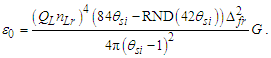 | (129) |
One must bear in mind that the description of G is a distance-sensitive property of the observer, not an intrinsic property of gravitation. Moreover, note that QLnLr=0.499983 at 42θsi and the differential Δfr=0.998158 both describe observational phenomena not intrinsic to the compared phenomena. The physical significance of that which describes their difference excludes the observer’s relative motion, and the distance is independent of the measurement-skewing effects between the inertial frame and the observed phenomenon.We now consider each of these ‘other phenomena’ that distinguish gravitation from electromagnetism, as follows.Two measurement-distortion phenomena: the metric and Informativity differentialsThe Informativity differential is described by QLnLr at 42θsi and the metric differential is described by Δfr. Each term describes a relative skew in measure. Importantly, the Informativity differential addresses the skew in lf with respect to the self-referencing frame. The metric differential addresses the skew in θsi with respect to the self-defining frame.First frame correlation: the metric differential associated with the fine structure constantGiven that the inverse fundamental fine structure constant is 42θsi, we then apply the metric differential to resolve the Planck equivalent as observed in the Measurement Frame. The expression is a function of the count of the base measure θsi corresponding to the charge coupling demarcation. | (130) |
Second frame correlation: the metric differential associated with elementary chargeThe terms below describe the metric differential associated with elementary charge. The expression may be considered a mathematical constant correlating the measure of e between the discrete and non-discrete frames; | (131) |
One particle/wave correlation: as a function of energyThe last term, found in the denominator, is 2π. As expressed in Eq. (116), the term may be described as the ratio of the energy of a fundamental unit of mass mf with respect to that of a photon; | (132) |
Collectively, the five expressions—all of which comprise mathematical constants—describe differences that distinguish the electric constant from gravitational curvature. With γ representing those terms that describe the skew in measure and geometries external to the intrinsic properties of the two phenomena,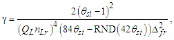 | (133) |
then the correlation of G to ɛ0 is | (134) |
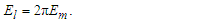
 | (135) |
As expected, the correlation follows the same form as for energy which carries no geometric component γ, El=2πEm.We advance one more expression with respect to energy. Arranging Eqs. (115) and (134) with both equaling 1/2π, we then set them equal yielding | (136) |
Thus, the gravitational constant corresponds to the energy of a photon as the electric constant does to the energy of mf, with γ describing the four additional geometries not intrinsic to the phenomena. We may also describe the energy Em of mf. Given El=2πθsic/QLnLr (Eq. 114) and θsi=QLnLrlfmf/tf, then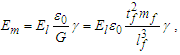 | (137) |
 | (138) |
 | (139) |
Although γ is a necessary part of the calculation, we consider it an external consequence of the geometry between the observer, the target, and the universe. When resolving the properties, the overall geometry is important to the calculation, but not relevant to the intrinsic properties of the phenomenon. Consequently, we consider the above energy expression a physically correlated function of the electric constant and fundamental measures, the remainder γ being geometric relative to our point-of-view. Notably, the extra fundamental units mf2/lf are precisely the base relative to θsi used to describe e. For instance, substituting mf2/lf with Eq. (94), then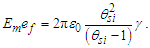 | (140) |
As such we find the product of energy and charge to describe one revolution and the electric constant, the remaining terms a function of the observer’s point-of-view.
3.5. Demarcations and Fundamental Constants
MQ allows us to use the physical correlation we have made between counts of θsi and that of α to do the same for Planck’s reduced constant. We clarify that one must choose to resolve values with the demarcation most appropriate to the phenomenon being described. We will use a discrete approach to the fine structure constant and then a second approach to resolve Planck’s reduced constant.The fine structure constant is defined against the Target Frame as αf−1=42θsi=137.020. When compared to the Measurement Frame, the value of α corresponds to the nearest whole unit count RND(nθθsi)=137. Hence, the quantization ratio is rq=137.020/137=1.00015. We express this as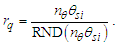 | (141) |
The ratio is a numerical description of the relationship between the non-discrete and discrete frames. Quantization ratios may also be defined by the inverse, but this relation has proved most useful.In that we are working with counts, which are nondimensional, the approach is both universal and applicable to all dimensions (i.e., θsi, lf). Importantly, the approach allows us to resolve α. However, before we begin, we briefly define some terminology (see Fig. 3).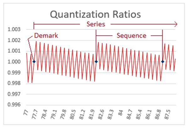 | Figure 3. Diagram of quantization ratio terms |
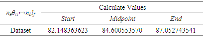
Demark—Given a plot of quantization ratios, there is a repeating pattern. Demark identifies the first point in each pattern such that y=1, with the average of a discrete set of points immediately to the left y<1 and the average of a discrete set of points immediately to the right y>1.Sequence—A plot of quantization ratios comprising points including both beginning and end demarks.Series—The set of sequences for which the beginning demarks share identical quantization ratios. A series may be distinguished as having a base demark nθ with repeating demarks such that each demark in the series is a whole unit count of the base (i.e., nθ: 42, 84, 126, …, 1050).Before we begin, we emphasize that quantization ratios are a function of discrete counts nθ of θsi, but we use those counts to resolve α with respect to the charge coupling demarcation, as a non−discrete multiplier nL of lf. A physical value is not needed, but we will need to map the pattern to a physical phenomenon, and we achieve this as a count of some measure. The two measures – θsi and lf – are correlated with respect to their count values such that nθ=RND(nL/2) as described in Eqs. (60) and (61). Moreover, resolving the midpoint—as is required for resolving the demarcation associated with α —produces the same value with any sequence to a considerable precision.Moreover, sequences are a function of the separation of data points along the x-axis (i.e., their quantization which is described by rq=nθθsi/RND(nθθsi), Eq. 86). Graph 1 is displayed with non-discrete x-axis values nθ incremented by 0.1 in separation. A 0.2 separation produces sequences that are half in length along the x-axis. A 0.3 separation produces a line that connects the upper left point of each sequence with its lower right point. Each may be used to obtain the same result, although larger separations of the data points become increasingly difficult to resolve. Importantly, the quantization separation is what produces the physically significant pattern that describes the charge coupling demarcation.Note also that different graphing programs will render differently. For instance, online tools such as desmos.com will not connect all the data points left to right as a continuous plot. Conversely, MS Excel does.Given the charge coupling demarcation is associated with a count of nθ=RND(nLr/2)=42, we may resolve the mid-point of that sequence near nθ=42 and then scale the count of lf with respect to the constant of proportionality. Or we may resolve the non-discrete mid-point of the sequence near nθ=84.9764 (Eq. 70) (i.e., any sequence may be used). To avoid scaling, we proceed with the latter. The demarcation count may be resolved relative to the midpoint of the second full sequence displayed in Graph I.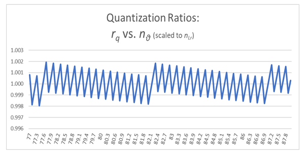 | Graph 1. Plot of Quantization Ratios Describing the Charge Coupling Demarcation |
Both the demarks and the halfway point fall on the y-axis with a value of 1 (Graph 1; also listed in Table 7). Points are resolved such that y=1 for the quantization ratio at the beginning, end, and middle of the sequence. Notably, what is being counted – θsi, lf, widgets – is irrelevant and affects only the magnitude of the quantization ratios along the y-axis. The resolution of the midpoint is a function of the x-axis count quantization, that is entirely a function of counting.Table 7. Metric Approach to Planck’s Reduced Constant
 |
| |
|
Such that nLrθsi=276, we find the charge coupling demarcation is nLr=276/θsi=84.6005.Conversely, we do not have an expression for Planck’s reduced constant with respect to the Target Frame. We can resolve its demarcation distance with Eq. (70). Knowing θsi and lf, then | (142) |
 | (143) |
 | (144) |
We will look at this more closely later with greater precision. But for now, we note that we can also write Eq. (143) as a function. Setting x=ħf/θsilf and y=1/nLr., we then have | (145) |
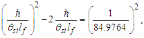
The solution as displayed in Fig. 4 for ħ/θsilf falls on the point (2.000069857, 0.000139718) on the right parabola. The axis of symmetry for both parabolas fall parallel to the x-axis. The expression can also be reduced. With ħf=2θsilf and ħ=θsilf/QLnLr, then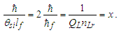 | (146) |
 | Figure 4. Skew in spatial measurement as a count of lf identifies the blackbody demarcation |
Substituting 1/QLnLr for ħ/θsilf, then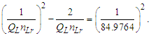 | (147) |
Thus, the x-axis describes the skew in measure between the non-discrete frame of the universe and the discrete frame of the observer, also known as the Informativity differential. The effect is geometric, independent of the rate of expansion (i.e., 2θsi, which is defined relative to the universe). The y-axis describes the blackbody demarcation. In that y is a function of x (i.e., f(x)=(x2−2x)1/2), it follows that the demarcation distance is also independent of the expansion—that is, independent of all system parameters particular to our universe. Both axes are dimensionless counts of lf.Although the expression is initially expressed as a function of Planck’s reduced constant, it can just as well be expressed as a function of θsi or several other physical constants. The relation does not describe the constants that make up the expression but describes the skewing of length relative to the Informativity differential.While the vertex of the right parabola corresponds to the blackbody demarcation, of interest is the vertex of the left parabola (positive in the x- and y-axes by a miniscule value). Is there a physical significance to this second property and will it be instrumental to understanding virtual particles? Do the two demarcations provide insight into the energy jumps associated with electrons? At this moment, we have established a new understanding of quantum phenomena, but how to translate these MQ descriptions is physically unclear.As a final note, Eq. (147) may be reduced given that nLr=84.9764 to resolve a blackbody demarcation of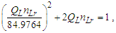 | (148) |
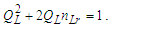 | (149) |
With this, we find that the Informativity differential is also a unity expression, just as Eq. (61), and describes the expansion of the universe in relation to the fundamental measures, each expression as described by the Pythagorean Theorem.
3.6. Metric Approach to Series of Sequences
As demonstrated with both the fine structure constant and Planck’s reduced constant, a metric approach can be used to identify physically significant values. In turn, those values describe physical characteristics of our universe, such as the quantum of action h and the ground state orbital of an electron a0. Moreover, there exists a physical correlation between the approach (i.e., frames of reference) and what we measure; in the case of ħ, we have an 11σ correspondence to its presently measured value. While the application of counts of fundamental measures to the description of constants is new, we may at least consider what additional properties may be deduced.Consider, for instance, not a specific count series (i.e., 42, 84, 126, ..., 42n, ...), but all count series of θsi. Among them, we look for repeating patterns in the quantization ratios. If the ratio values repeated indefinitely or were not otherwise constrained, they would be uninformative. However, there are constraints to the relationships that may exist. That is, the quantization ratios associated with each demark repeat up to a certain point. The corresponding series for the first 64 counts are listed in Table 8.Table 8. Repeating quantization ratio demarks for counts nθ up to 64
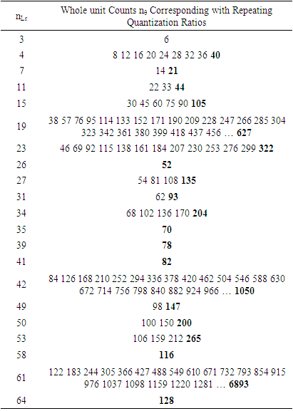 |
| |
|
A quantization ratio rq is calculated such that rq=nθθsi/RND(nθθsi). By example, consider the fine structure constant, which we have shown to be physically correlated with a count of 42. The quantization ratio is then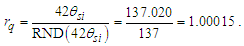 | (150) |
Carrying the operation out for each count … 1, 2, 3, 4, 5 … we can then compare the quantization ratios for matching values. In the case of the 42 series, there are matching ratios at nθ equal to 42, 84, 126, 168 … 42n … 1050. There are no more matching values above or below a series. This series is physically correlated to the fine structure constant, to Planck’s constant, to the blackbody demarcation, and by means of these constants to other phenomena.With respect to these results, we pose several questions.Why are all discovered phenomena associated with the 42 count series?Such that the count nθ=42 identifies the series that corresponds to the fine structure constant and our understanding of the quantum of action, we find also that the first count value identifies the x-axis value associated with the charge coupling demarcation. Moreover, we find that, adjusted for measurement skewing described by the metric and Informativity differential, a count of 42 θsi may be used to identify the ground state orbital a0 of an electron. With these and other physical correlations, we may inquire if there is something unique to this series that all values thus far are physically correlated with only this series.Are there physical constants that are independent of the fundamental measures?Had the rate of expansion for our universe been something other than 2θsi, would that change some or all properties of the universe? Recall that quantization ratios are a function of fundamental measures and counts. Count properties such as the charge coupling demarcation and the Informativity differential are geometric, independent of the rate of expansion. For this reason, there exists a path to realize that some physical constants, and as such some phenomena, although they may differ in value, will exist regardless of the system parameters of our universe.Are discrete systems the cause of breaks in physical symmetry?Importantly, we note that a non-discrete universe would be symmetrically equal. However, a non-discrete universe with no external reference creates a discrete internal frame of reference. This leads to asymmetries; for instance, comparing counts of sequences starting with odd x-values (there are 21) to those starting with even x-values (there are 7) of the first 64 whole-unit values (see Table 8). It is conjectured that this lack of symmetry in discrete systems is the source of physical variations we observe in nature.O8: A universe with no external frame of reference will not be symmetrical in all aspects.We focus on the metric approach to consider whether both the geometry and the counts of fundamental measures are important when describing observed phenomena. For instance, consider a mass divided into three equal parts; the physical properties of the parts are affected by the division, many of those properties being a straight-forward division by three. For example, the effects of gravitation from each part are now one-third of the original whole.From another perspective, SR may be viewed as a geometric phenomenon that is consistent with certain numerical properties. That is, there are specific consequences to the observation of length, mass, and time relative to the numerical increase or decrease in velocity between the observer and target. For this reason, an investigation of the permitted counts associated with the description of phenomena is important.
3.7. Extending Precision of the Physical Constants
Using the metric approach, we were able to resolve values of several physical constants. For example, we resolved the fine structure constant as a count of θsi. Unfortunately, θsi is constrained to six digits of physical significance. Here, we reverse the calculation resolving a more precise value of θsi as a measure of the magnetic constant and the charge coupling demarcation ‘distance’ in the Target Frame, | (151) |
The expression is an essential observation that can be validated for any given count nθ and corresponding θsi such that rq=1, nLrθsi=276. The value corresponds to αc-1 defined with respect to the Target Frame. With this we may resolve the immeasurable distance associated with α. | (152) |
 | (153) |
 | (154) |
Using the 2018 CODATA value for αc=7.2973525693 10-3 [1] then,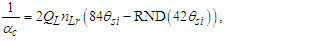 | (155) |
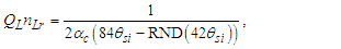 | (156) |
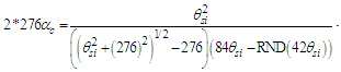 | (157) |
 | (158) |
Notably, a recent study resolves α to 81 parts per trillion, α-1=137.035999206(11) [18] with respect to the recoil velocity of a rubidium atom that absorbs a photon. This measure demonstrated a strong disagreement with calculated values for αp (a difference of 1.28 10-11 greater than the presently accepted CODATA value of α-1=137.035999084 (21) [1]) suggesting that measurements of the cesium atom demonstrate a stronger correlation to the fine structure constant. Morel, L., Yao, Z., Cladé, P. et al. Determination of the fine-structure constant with an accuracy of 81 parts per trillion. Nature 588, 61–65 (2020). https://doi.org/10.1038/s41586-020-2964-7.The charge coupling demarcation associated with the fine structure constant is then,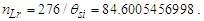 | (159) |
 | (160) |
The corresponding Informativity differential is at | (161) |
In addition to the quantum entanglement correlation, we now offer this second approach to the measurement of θsi. Using the expression for mf from Eq. (37), then | (162) |
The remaining two measures, lf and tf are functions of G constrained to six digits. However, we may use Planck’s formula for the fine structure constant (Eq. 63) to resolve lf. We must also solve αp−1 as a function of the new θsi. | (163) |
Now with mf and αp as a function of the new value for θsi and with which the remaining values are measured, then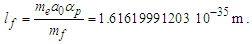 | (164) |
We use αp over αc in recognition that Planck’s expression should not be adjusted for the Informativity differential as demonstrated in Eq. (69). In turn, using the defined value for the speed of light leads to a value for fundamental time.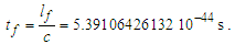 | (165) |
In that the value of c is defined we have interpreted this to have no effect on the precision of the result. Continuing, the gravitational constant when measured macroscopically is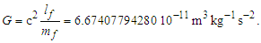 | (166) |
Moreover, the value of ħ such that all values derive from the measure of μ0, the blackbody demarcation nLr and c is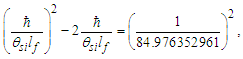 | (167) |
 | (168) |
The value of αc from Eq. (156) is defined as a function of ħ, which makes this last calculation significant only for measured values of α not a function of ħ (i.e., αc=cμ0/2RK such that μ0 is measured directly). Moreover, to calculate a distance sensitive value that accounts for the Informativity differential we use the expanded form. We may, for instance, resolve ħf at the upper count bound. This value is approximately accurate for any macroscopic measurement. | (169) |
 | (170) |
There is always a series of measures that underpin each calculation. Our initial measure of θsi comes from the 2018 CODATA definition of αc which depends on the measure of μ0. The electric constant is also a function of μ0 with ħ, e, and c being defined. As such, we cannot use our more refined values to then calculate elementary charge, the electric or magnetic constants. Doing so would create a loop. But we can improve our electromagnetic calculations.Recall that we needed to apply the differential after resolving an expression for the metric differential. This approximation is wholly contained within γ. With our new expressions for the electromagnetic constants, we can isolate gamma with respect to the measure of each constant independently. | (171) |
 | (172) |
 | (173) |
Notably, the value of γ is the same for all three measurements. Such that the most appropriate measurement is used for each solution, then | (174) |
 | (175) |
 | (176) |
We compare these results in Table 9.Table 9. Electromagnetic constants as a function of the fundamental measures and γ
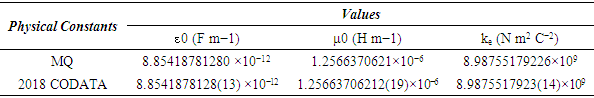 |
| |
|
There are many values that may be described as a combination of these, now with more precise results. For instance, the ΛCDM distributions are now resolvable ([11], Eqs. 82-86) to twelve digits of physical significance,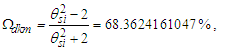 | (177) |
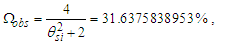 | (178) |
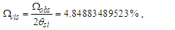 | (179) |
 | (180) |
Lastly, some values in this paper quote the 2010 CODATA results. There have been changes in the 2018 measure of G reflecting new measurement techniques that are more subject to the effects of the Informativity differential. That is, there are calculated values, some terms measured macroscopically while others measured quantumly. As such, we have endeavored to use measures that are least affected by the Informativity differential.
3.8. Particles vs. Waves
We have provided expressions that correlate particle and wave phenomena. Invariably, they differ by a constant, 2π. What does this describe? Why are there so many phenomena that differ by this value? And what is the physical significance of this difference? The answers to these questions are at the heart of particle/wave duality. They arise from a geometry that underlies the universe.To better grasp the scope of physical phenomena that differ by this value we will review. Firstly, consider energy, that is the energy of a fundamental unit of mass mf and a corresponding quantum of light ([7], Eqs. 48-51). | (181) |
 | (182) |
 | (183) |
 | (184) |
Their difference is 2π. Moreover, n is not a whole unit value, at least not in terms of counts. Written using Planck’s expression E=nhv, we find that n is 1/2π when describing mass. Therefore 2π appears in expressions describing electromagnetic phenomena.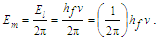 | (185) |
Note also that expansion of the expression to describe the energy of light reflects Einstein’s equation E=mc2. Such that El=2πEm (Eq. 184) and Em=2θsic (Eq. 182), then 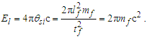 | (186) |
Importantly, the value of 2π is what distinguishes the energy of mass mf from that of light. Consider now the phenomenon of force. This relation, resolved earlier in the paper, describes how gravitation and electromagnetism are correlated. | (187) |
Once again, the two phenomena are separated in value by 2π. Gamma, incidentally, is used to indicate four geometries instrumental to the calculation, but not representative of the intrinsic properties of either phenomenon. Consider now the CMB power spectrum. As presented in Appendix F, we observe that the x-axis coordinate of the peak of each curve is distinguished as a function of π.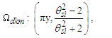 | (188) |
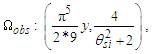 | (189) |
 | (190) |
 | (191) |
 | (192) |
This is not unexpected with electromagnetic descriptions, but we have demonstrated that these descriptions are temporal in origin. Moreover, there is a relativistic offset. Applying the offset to each x-value, | (193) |
we account for the skewing effects of measure between the earliest and present epochs ([11], Eq. 90).Let us now consider what a particle is in terms of energy. The energy of a fundamental unit of mass is Em=2θsic. Notably, such that 2θsi is the rate of universal expansion HU and c is the velocity of all points relative to observers at the visible bound – a system perimeter, that spacetime where there is no information beyond the bound, we find that Em is the product of the expansion parameter and the perimeter velocity.  | (194) |
What, then, is mass? What is the relation between mf and a universe? Is there a greater physical significance to π? | Figure 5. Arc length of a circle of radius lf, subtending angle θ radians |
That is, we bring together a suite of phenomena each which carry the value of π across multiple disciplines: energy, gravitation, electromagnetism, cosmology, and epochs. We correlate them, demonstrating that it is π which stands between them. Yet, we also describe π as a geometry reflective of a description of a circle. As described in Fig. 5, such that the circumference of a circle is C=2πr, it is that geometry which describes this difference as a ratio, the circumference divided by the radius. Moreover, given the radius of a circle equal to lf, we find that the radian measure θsi corresponds to half of a quantum of energy ħ/2, again h divided by 2π (i.e., C/r). We typically refer to this as its angular momentum. From each of these observations, we may observe thatO9: Phenomena come in pairs separated in value by 2π.In all cases, we find it an inevitable conclusion that energy, mass, and force each present themselves in pairs, partner phenomena separated by a geometry of 2π, C/r.
3.9. Singularities
Singularities in modern theory are encountered in situations such as General Relativity (GR) [19] when used to describe phenomena at the extreme of the measurement domain (i.e., the center of a black hole or the universe as a quantum singularity).Notably, MQ is a discrete nomenclature, a physically significant description of phenomena as counts of three fundamental measures, lf, mf and tf. In that there are no fractional counts of physical significance in the Measurement Frame, there are no opportunities for singularities. The value of any count in an expression starts with one and has an upper bound which does not exceed the Planck frequency, 1/tf.A demonstration of the issue as occurs in GR may be better understood in analysis of the expression for escape velocity ve. Consider the velocity bound such that v=c. Then | (195) |
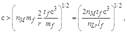 | (196) |
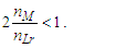 | (197) |
We recognized that the observer and the target cannot both occupy the same space at the same time. Thus, the count value for nLr must be greater than 0. Moreover, nLr must be greater than two times nM, nM also greater than 0. To correlate this to relativity, the measurement distortion expressions ([8], Eqs. 31-34) also described by SR are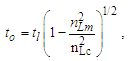 | (198) |
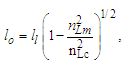 | (199) |
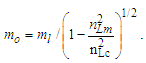 | (200) |
The counts correspond to their classical counterparts such that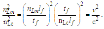 | (201) |
And using the escape velocity expression, then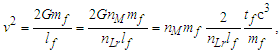 | (202) |
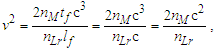 | (203) |
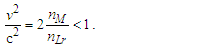 | (204) |
Their mathematical and physical equivalence are then demonstrated by their combination. Notably, the presentation is intentionally simplistic. A more exhaustive presentation is available in the second paper, ‘Measurement Quantization Unifies Relativistic Effects …’ [8]. | (205) |
We find then, no opportunity for a speed parameter in relativistic expressions to present singularities. All descriptions of phenomena must satisfy nLr≥1, nM≥1 and nT≥1 such that all counts are whole unit. The root cause of singularities arises as a by-product of a non-discrete nomenclature when describing phenomena. MQ recognizes the physical significance of discrete measure and respectively modifies modern nomenclature with a more precise terminology. Physically significant bounds are then more easily recognized. This physically significant rule set does not allow singularities and preserves an understanding of the properties that underlie what is being described.
4. Discussion
In this paper, we use MQ to resolve physically significant descriptions of the constants of nature. We developed a foundation for their origin—a differential between the discrete framework of the observer and the non-discrete framework of the universe—and various relations, variations of the fundamental expression. Importantly, we complete a picture of what were formally unanswered questions: Why do the physical constants exist? Why do the laws of nature exist? Why is the universe symmetrical and where is it nonsymmetrical? Why does the use of classical mechanics present singularities?While these questions were at some point intangible, we now look to new questions. Why is the blackbody demarcation at 42θsi? Why is the fine structure constant a function at 42θsi? Why is Planck’s expression for α a differential of the fine structure constant, a function of 42θsi? And finally, why is the ground state orbital of an atom a function of 42θsi?A review of Table 8 offers some possibilities. If starting values are conjectured to be based on orbitals for the atom (which then need adjustment for the effects of force), it follows that the universe might have corresponded to any count series, for example, 41θsi or 39θsi. However, these series afford only two orbitals for atoms. It may also be conjectured that there is no preferential series. The universe could have just as easily corresponded to the 19θsi or 61θsi count series. This leads to the question, why are there so many odd count series compared with even, 21 to 7 for the first 64 whole-unit counts? Is this lack of symmetry at the root of the matter/anti-matter differential? These questions are purely speculative, intended to spark interest for further investigations. Conversely, the presentation addresses only verifiable results with straight-forward physical correlations.Among other discoveries, the greatest challenge we have encountered is a better understanding of unification. We may agree that unification involves a description of each phenomenon correlated with an equality. In that the phenomena are physically distinct, there will be some count of additional phenomena that distinguish them. Nonetheless, as demonstrated in Eqs. (105)–(108), it is easy to correlate phenomena and identify other phenomena that distinguish them. Thus, a more fundamental definition is needed.Perhaps unification requires a shared fundamental nomenclature and physically significant distinct terms independent of the correlated terms. Perhaps some element of naturalness and/or elegance is prerequisite to the solution. Are these the ground rules for unification? If agreed, then have we completed unification of the four forces or are we just beginning? We should consider the latter.Finally, the attentive reader will note that there is no intent to push geometry into the spotlight. The correlation of so many phenomena to numerical qualities is not our focus. We emphasize, as has long been the tradition of science, that finding the best math that describes the world around us is our greatest endeavor. That more of nature appears geometric is irrelevant.
5. Glossary of Terms
Blackbody demarcationThat distance at 84.9764lf, (Appendix D) corresponding to the measure of blackbody radiation, the value of QLnLr=0.499996 and the value of ħ as we recognize it today.Charge coupling demarcationThat distance at 84.6005, corresponding to the measure of the fine structure constant and the value of QLnLr=0.499996. Fundamental expressionThe simplest expression that relates the three measures, length lf, mass mf, and time tf. The expression is lfmf=2θsitf such that the value of θsi is 3.26239.InformativityA field of science that recognizes the physical significance of nature as a consequence of mathematical form. We use Measurement Quantization (MQ) as an approach to describe the discrete properties of nature revealing how nature and mathematical form are correlated. This is achieved with a nomenclature of counts of physically significant fundamental units of measure applied to the existing classical laws of modern theory. Notably, MQ is just one approach. Other approaches are likely to arise specific to quantum theory, information theory and high energy physics. Regardless of the approach, we identify the science of Informativity as any discipline that recognizes the constants and laws of nature as a consequence of mathematical form.Informativity differentialA skewing of the measure of length because of the discreteness of measure. The effect is geometric and may be described as a count of lf such that QLnLr=((1+nLr2)1/2-nLr)nLr. QL is the non-discrete count of lf that is lost at each count of tf with respect to elapsed time. This effect is known as gravity, although the differential itself is also recognized as a skewing of measure in a fashion like relativity, except with respect to distance, not motion.Metric differentialFollows the same geometric displacement described by the Informativity differential but is calculated as a difference between a discrete and non-discrete count n of a fundamental measure.RNDThe term RND is used often in MQ and meant to describe a physical process whereby the measure of an object at a non-discrete distance appears to be at the nearest count of a fundamental measure. Thus, if a calculated value has remainder less than one half, the lower count is measured. If a calculated value has a remainder greater than one half, the upper count is measured. A calculated value with a remainder equal to one half has an uncertain count value, either above or below the non-discrete value. Counts apply to all dimensions, but with respect to distance all calculated values are less than one half and as such round down.Self-referencingAn expression defined with respect to the observer’s inertial frame of reference.Self-definingAn expression defined with respect to the universe as a frame of reference.System parametersAny constant value associated with a self-defining expression (i.e., θsi).MQ nomenclatureA nomenclature of all fundamental units of measure—lf,, mf , tf, and θsi—which are discrete, countable, and may be used exclusively to describe all observed phenomena in the universe. The acronym MQ stands for measurement quantization. The nomenclature is applied to the well-tested and strongly supported laws of classical mechanics.Quantization ratioThe ratio is a numerical representation of the relation between the discrete and non-discrete frameworks, a function of the count n of a fundamental measure, typically θsi or lf. The ratio nθsi/RND(nθsi) is defined with RND(*) denoting the value of the argument rounded to the nearest whole-unit.Demark—Given a plot of quantization ratios, there is a repeating pattern. Demark identifies the first point in each pattern such that y=1, with the average of a discrete set of points immediately to the left y<1 and the average of a discrete set of points immediately to the right y>1.Sequence—A plot of quantization ratios comprising points including both beginning and end demarks.Series—The set of sequences for which the beginning demarks share identical quantization ratios. The series may be distinguished as having a base demark B with repeating demarks such that each demark in the series is a whole unit count n of the base (i.e., nB: 42, 84, 126, …, 1050).FrameworksReference framework—This is the framework of the observer. With respect to the traditional understanding, this framework differs only in that measure is a count function of discrete length measures equal to one. It shares those properties of the self-referencing frame of reference but in relation to the inertial frame of the observer.Measurement framework—This framework shares properties with the Reference Framework. It is characterized as some known count of the reference length measure.Target framework—This framework is characterized by the property of measure of non-discreteness, that being the framework of the universe that contains the phenomenon. It shares those properties of the self-defining frame of reference but in relation to a local phenomenon.Self-referencing frame of reference—A system of geometric axes anchored with respect to objects within the universe to which measurements of size, position or motion can be made. One may assign expressions comprising physically significant terms. However, those terms are defined with respect to other terms (i.e., ħ, ɛ0, μ0, α, lf, mf, tf) such that there exists no external anchor with which to resolve any term independently.Self-defining frame of reference—A system of geometric axes anchored with respect to the universe to which measurements of size, position or motion can be made. One may assign expressions comprising physically significant terms. Those terms, also known as system parameters, are defined numerically with respect to properties of the universe (i.e., rate of universal expansion 2θsi, age of the universe AU), but have no relation with respect to phenomena external to the universe.
ACKNOWLEDGMENTS
We thank Edanz Group (www.edanzediting.com/ac) for editing a draft of this manuscript.
Appendices
APPENDIX A: INFORMATIVITY DIFFERENTIAL QLnLr ([11], Appendix A)In analysis of Heisenberg’s uncertainty principle, we resolve properties of measure demonstrating discreteness, countability and in relation to three frames of reference. Notably, the physical significance of discrete measure also demonstrates that there is a skew between such a description and that of an expression not constrained by a whole-unit count of fundamental measures. We find that difference best described by QLnLr and refer to this term as the Informativity differential. Resolving the limits to QLnLr is valuable when working with MQ expressions.We approach this goal by recognizing that the product of QLnLr (Eqs. 30 and 31) is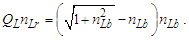 | (A1) |
Recall that there are three frames involved in a description of measure, such that Side a is the reference count nLa, Side b is some count nLb of that reference and Side c is the measured count, such that nLc=nLr+QL and nLb=nLr. Such that we wish to describe Side c, we drop the nLb term and adopt the term nLr in that r is more commonly associated with the measure of distance.We verify that nLb=nLr such that the highest value for QL is nLb=1 where (1+12)0.5–1≈0.414 and the ‘observed’ distance of Side c – a count nLc of lf – is always rounded to the nearest integer value. That value is equal to the count nLr. It is QL=√2-1 at its highest and quickly approaches 0 with increasing nLr.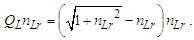 | (A2) |
At the lower limit nLr=1, then limr=1f(QLnLr) =√2−1. Conversely, dividing by nLr, adding nLr, squaring, subtracting nLr2, and dividing by 2, we find that the upper limit is | (A3) |
In analysis of this expression, we recognize with increasing nLr that QL decreases to 0. The left term drops out such that the Informativity differential QLnLr approaches 0.5. At 2,247 lf the value of QLnLr rounds to 0.5 to six significant digits, with no difference in the ninth digit at 104 lf.APPENDIX B: MEASUREMENT OF θsi ([11], Appendix B)In addition to a physical correlation of θsi with measure of the magnetic constant (Eq. 157), we have correlated θsi in value with respect to X-rays in maximally entangled states as described by Bell. Measurements were taken by Shwartz and Harris and published in their 2011 paper [3]. Within it, they also offer a model that describes their results.We will now describe a second dimensional quality of θsi, a numerical correlation in its value as a momentum with respect to the angle of polarization of X-rays when satisfying a maximally entangled Bell state. Correlated to the lattice vector  two vectors are described: one, a polarization of the electric field in the scattering plane and two, the polarization of the electric field orthogonal to the scattering plane. This new approach allows us to offer a new expression for θsi such that the two vectors differ in sign, a division of the magnitude of the coordinate components of the pump wavevector. Thus, the x and y components are respectively the arccosine and arcsine of the lattice vector and may be described as (−npxcos(θ), npysin(θ)). With this we resolve the magnitude of each vector, the pump, signal and idler. We denote the vectors (a function of the pump frequency or the phase matching properties of the nonlinear optical crystal) with the symbol n and distinguish the signals with the subscript p, s or i. To identify the coordinate axes, we add an x or y.
 | (B1) |
 | (B2) |
The component vectors yields are then | (B3) |
 | (B4) |
 | (B5) |
 | (B6) |
We complete the reduction in three steps. First, we move the pump coordinate to the right alongside the lattice vector. We then take the angular difference of the y-component to make the sine positive. And finally, we match the form found in the x-component. | (B7) |
With this we resolve that θs=θi. Notably, we also see that the pump angle is θp=2π−θ. And such that the pump is split evenly, we recognize that the momentum of the beam is divided. Thus, the angles of the k vectors with respect to the atomic pane must equal half the momentum of the entangled photons (i.e., S). Such that θsi=mflf/tf, then | (B8) |
Referring to the Shwartz and Harris model, we recognize that one additional data row may be resolved also using this approach. Using Eq. (B5) as described in line 2 of Table 10, we recognize that the respective angles for the signal and idler are precisely a function of the measure at maximal entanglement θMax. And by subtracting each angle from π (i.e., π−θp, π−θs, π−θi) we resolve line 1.Table 10. Predicted radian measures of the k vectors of the pump, signal and idler for the maximally entangled polarization at the degenerate frequency of X-rays
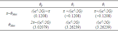 |
| |
|
In Table 11, we describe the Shwartz and Harris projections with respect to two of five Bell states they identify as generating entangled photons. For consistency, we also adopt their nomenclature, such that |H> is the polarization of the electric field of the X-ray in the scattering plane and |V> is the polarization orthogonal to the scattering plane, which contains the incident k vector and the lattice k vector 
Table 11. Angle setting in radians of the k vectors of the pump, signal, and idler for maximally entangled polarization states at the degenerate frequency [3]
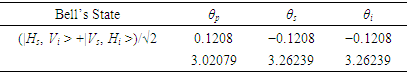 |
| |
|
The MQ descriptions match the Shwartz and Harris measures to six digits, the extent with which each model has physical significance. Notably, with respect to the measurement data, Shwartz and Harris note that the error in measure is less than 2 micro-radians.On top of the correlation already presented between gravitation and electromagnetism, the Shwartz and Harris correlation continues to add to our physical understanding of θsi as having a distinct measurable value but differing dimensional qualities as a function of the phenomenon being measured. In this case, we find angular measure correlated to the scalar constant S=lpc3/2G, a composition of the fundamental length lp, the speed of light c, and the gravitational constant G. By demonstration only, using the 2010 CODATA [2], the calculation matches the Shwartz and Harris results.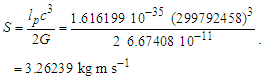 | (B9) |
As noted previously in this paper, newer approaches to the measure of G reflected in the 2014 and 2018 CODATA are affected significantly by the Informativity differential. For this reason, we consistently adopt comparisons with the 2010 CODATA when discussing measures that include G.APPENDIX C: FUNDAMENTAL MEASURES ([10], Sec. 3.4)We may resolve the fundamental measures using only our initial observations regarding an MQ description of quantum gravity and its relation to Newton’s expression for G. Such that G/r2=QLc3/rθsi (Eq. 34), then factoring out the Informativity differential limnLr→∞f(QLnLr)=1/2 (Appendix A) we resolve that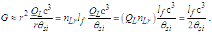 | (C1) |
Given that G=c3tf/mf (Eq. 16), then | (C2) |
 | (C3) |
We identify this as the fundamental expression. Notably, we can also resolve the expression from Eq. (34), but this assumes a physical correlation with respect to the Newton description. Thus, we start with Eq. (33) and resolve that G=c3tf/mf as a physically significant description with respect to our expression of quantum gravity. This may then be extended. Such that the Informativity differential limnLr→∞f(QLnLr)=1/2, then | (C4) |
 | (C5) |
 | (C6) |
 | (C7) |
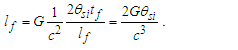 | (C8) |
For all macroscopic distance, the fundamental measures are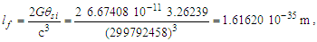 | (C9) |
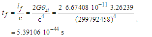 | (C10) |
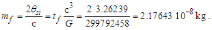 | (C11) |
APPENDIX D: BLACKBODY DEMARCATION ([10], Appendix B)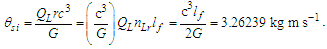 | (D1) |
We have substitute ħ/lf2 from Planck’s relation (Eq. 1). Thus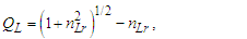 | (D2) |
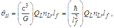 | (D3) |
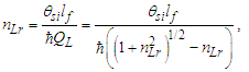 | (D4) |
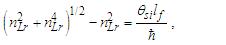 | (D5) |
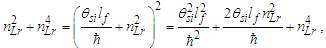 | (D6) |
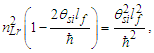 | (D7) |
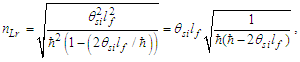 | (D8) |
 | (D9) |
APPENDIX E: OBSERVABLE MASS BOUND ([9], Appx. 5.3)In classical theory we recognize that no phenomenon may have a relative change in position greater than the speed of light. When we apply a MQ nomenclature to a description of relative motion, we would characterize such a change as an ‘observed measure count’ of lf per count of tf. Within the field of classical theory, such concepts are commonly recognized although the Planck Units have no known physical significance.With this presentation, we add to our understanding of nature that the fundamental units are physically significant. Counts of the fundamental measures are important and give rise to the properties and characterization of observed phenomena. It is with this understanding that we recognize there also exists an upper ‘observed measure count’ of mf per count of tf. We call the upper count bound of lf to tf the length frequency. We call the upper count bound of mf to tf the mass frequency. Developing an expression that describes these phenomena may at first seem straight-forward, but when accounting for the relative view of an observer in a spacetime, it becomes more complex. There are several questions that one can engage to untangle why.Such that the count of mf has an upper count bound, what happens when the observable mass exceeds this bound? Does that mean that the excess mass is invisible? And what expressions describe a mass distribution that is uneven, for instance, an observer in a galaxy? These questions are central to understanding dark matter and are discussed in this paper, ‘Measurement Quantization Describes Galactic Rotational Velocities …’ [9]. For our needs, we will resolve only an expression describing observable mass. This will allow us to resolve the relation between mass and time at the bound c.Such that G=c3tf/mf, then the escape velocity is equal to the classical velocity bound at c.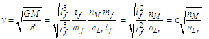 | (E1) |
The mass-to-length count bound with respect to the escape velocity is then | (E2) |
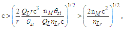 | (E3) |
 | (E4) |
Notably, the smallest count of mf with respect to lf may not be less than the precision of the reference mf=2.17647x10⁻⁸ kg. Then,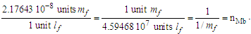 | (E5) |
Correlating both bounds the ratio is then 2 units of mf per unit of lf such that 1/(1/mf). Thus, 2(1/(1/mf))=2mf. Moreover, such that nMb and mf are equal in value without units, then the classical velocity bound is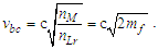 | (E6) |
The expansion of space HU=2θsi ([9], Eq. 27) is not included in the expression. Given that HU is relative to the diameter of the universe, divide by 2. Then, the radial expansion respective of orbital and escape velocity vb may be written in two ways. The fundamental expression may be used to convert between them.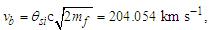 | (E7) |
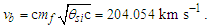 | (E8) |
Both θsi and our substitution of mf for nMb carry no units. The expression describes the velocity bound corresponding to the upper count bound of mf that may be discerned at a point in space. The corresponding mass bound is then vb equal to the same as expressed with Newton’s expression. 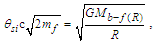 | (E9) |
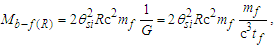 | (E10) |
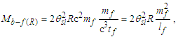 | (E11) |
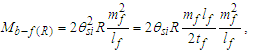 | (E12) |
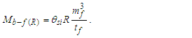 | (E13) |
We observe that mf in Eq. (E9) is a dimensionless substitute for nMb. There are no units. But, in Eq. (E12) where R in meters cancels with lf in meters, we are left with mf2 and a single kilograms describing Mb-f(R). But in Eq. (E9) we introduced the fundamental expression θsi=lfmf/2tf. Cancellations leave both R, tf and an additional mf dimensionless. The result is kilograms, | (E14) |
APPENDIX F: POWER SPECTRUM DISTRIBUTIONS ([7], Sec. 3.11)Before we begin, there exists a significant question regarding the value of the cosmological constant. New insights into its value may be resolved when considering Einstein’s observation that the speed of light is constant for all observers. We extend this observation to recognize all frames of reference for which an observer may consider.It follows that the upper bound rate nL/nT of lf per tf at which two phenomena may regress with for all inertial frames, including those considered at the leading edge of a system, must equal c. Moreover, the relation between length and time in the Measurement Frame is described by the fundamental expression. | (F1) |
But, as we recognize, the speed of light is constant for all observers in consideration of all frames. Thus, in addition to the observer’s Measurement Frame, light is also constant as described with respect to the observer’s Target Frame. This implies that,O10: Any measure other than that described by the fundamental expression would describe observers that observe a speed of light other than c.We also recognize that the universe as defined by that space traveled by light since the Big Bang is physically significant. This does not mean that matter occupies all space in the Target Frame of all observers. We recognize that the presence of mass may differ from the space described by the fundamental expression when defined relative to the Target Frame and as such distinguish universal expansion (i.e. the expansion of the universe) from stellar expansion (i.e. the expansion of galaxies away from one another).Replacing distance and elapsed time as used in the Measurement Frame with those terms corresponding to the Target Frame nTtf=AU, nLlf=DU (i.e. the diameter DU and age AU of the universe), then | (F2) |
 | (F3) |
 | (F4) |
To break down the terms in the parenthesis, we note that mf=2θsi/c when defined with respect to the Target Frame follows c=nLulf/nTutf=(nLu/nTu)c. Thus, | (F5) |
But as there exists no reference for mu external to the universe, we recognize that mu=1 in the Target Frame of the universe, a self-defining unity expression. We may then organize terms on the right side of the equality such that | (F6) |
 | (F7) |
Now, with the fundamental expression describing the relation between each dimension as a function of the Measurement and Target Frames, we may reduce the terms in the parenthesis of Eq. (F4) to resolve that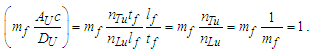 | (F8) |
Given an age of the universe equal to 13.799±0.021 billion years [5], then | (F9) |
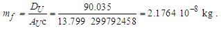 | (F10) |
Notably, the same ‘unity’ arguments may be made with respect to length and time, but unlike that made with respect to mass, such that the relation between the remaining dimensions length and time (i.e. c=lf/tf) is a known constant, the relation between time and mass as well as mass and length are not so easily measured. It is only because of the known value of c that this argument can be carried out. Moreover, note that the constancy of c for all observers is reflected in c=(DU/AUmf) (Eq. F10) such that DU/AU describes the rate of universal expansion. Thus,O11: Physical support for the constancy of light in all frames exists only in a flat universe.O12: The rate of universal expansion when defined with respect to the system is constant, DU/AU=cmf=6.52478 ly/y.With this, we may then approach a description of the universe as a function of the system volume (i.e., as described by the fundamental expression) and the critical density defined with respect to that space. Such that VU=(4/3)πRU3, G=c3tf/mf from (Eq. 16), RU/AU=θsic ([11], Eq. 44), and where the critical density of a flat universe ρc=Hf2/8πG [20] is a function of the Hubble frequency ([7], Eq. 60), then | (F11) |
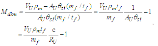 | (F12) |
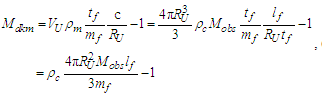 | (F13) |
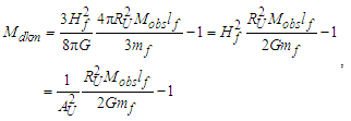 | (F14) |
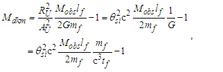 | (F15) |
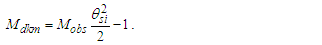 | (F16) |
Organizing this expression in combination with the observation that the sum of the dark and observable distributions must equal 1, then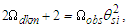 | (F17) |
 | (F18) |
We may combine the two expressions to resolve their distribution values.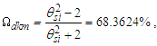 | (F19) |
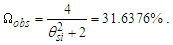 | (F20) |
Finally, such that the leading edge of the universe is expanding at the speed of light vU=c and such that 2θsic defines the ratio of the observable relative to the visible Mobs/Mvis (i.e., two times the RU/AU=θsic referenced in the first paragraph) we may use these constraints to resolve the remaining distributions. Note, Ωtot=1; as such, the term may be dropped.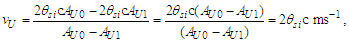 | (F21) |
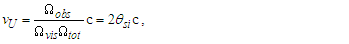 | (F22) |
 | (F23) |
 | (F24) |
References
| [1] | NIST: CODATA Recommended Values of the Fundamental Physical Constants: 2018, (May, 2019), https://physics.nist.gov/cuu/pdf/wall_2018.pdf. |
| [2] | P. Mohr, B. Taylor, and D. Newell: CODATA Recommend Values of the Fundamental Physical Constants: 2010, p. 3, (2012), DOI: http://dx.doi.org/10.1103/RevModPhys.84.1527. |
| [3] | S. Shwartz, and S.E. Harris: Polarization Entangled Photons at X-Ray Energies, Phys. Rev. Lett. 106, 080501 (2011), arXiv: 1012.3499. |
| [4] | Planck Collaboration, Planck 2013 Results. XVI. Cosmologi-cal Parameters, Astronomy & Astrophysics, 571 (2013). |
| [5] | Planck Collaboration, Planck Collaboration 2018 Results VI (2018), [arXiv:1807.06209]. |
| [6] | M. Planck, Über irreversible Strahlungsvorgänge, Sitzungsberichte der Königlich Preußischen Akademie der Wissenschaften zu, Berlin, 5, p. 480 (1899). |
| [7] | J.A. Geiger: Measurement Quantization Unites Classical and Quantum Physics, Journal of High Energy Physics Gravitation and Cosmology. Vol. 4, No. 2, 262–311 (Apr 2018). https://doi.org/10.4236/jhepgc.2018.42019. |
| [8] | J.A. Geiger: Quantum Model of Gravity Unifies Relativistic Effects, Describes Inflation/Expansion Transition, Matches CMB Data, Journal of High Energy Physics Gravitation and Cosmology. Vol. 4, No. 4 (Oct 2018). https://doi.org/10.4236/jhepgc.2018.44038. |
| [9] | J.A. Geiger: Measurement Quantization Describes Galactic Rotational Velocities, Obviates Dark Matter Conjecture, Journal of High Energy Physics Gravitation and Cosmology. Vol. 5, No. 2 (Apr 2019). https://doi.org/10.4236/jhepgc.2019.52028. |
| [10] | J.A. Geiger: Physical Significance of Measure, Journal of High Energy Physics Gravitation and Cosmology. Vol. 6, No. 1 (Jan 2020). https://doi.org/10.4236/jhepgc.2020.61008. |
| [11] | J.A. Geiger: Measurement Quantization Describes History of Universe – Quantum Inflation, Transition to Expansion, CMB Power Spectrum, Journal of High Energy Physics Gravitation and Cosmology. Vol. 6, No. 2 (Apr 2020). https://doi.org/10.4236/jhepgc.2020.62015. |
| [12] | G. Stoney, On the Physical Units of Nature, Phil. Mag. 11. 381 - 391 (1881). |
| [13] | Wesson, P. S. (1980). The application of dimensional analysis to cosmology. Space Science Reviews. 27 (2): 117. Bibcode: 1980SSRv...27..109W. doi:10.1007/bf00212237. S2CID 120784299. |
| [14] | Petr. Křen, Why dimensionless units should not be used in physics (2019). https://arxiv.org/abs/1911.10030. |
| [15] | L. E. Ballentine, The Statistical Interpretation of Quantum Mechanics, Rev. Mod. Phys. 42 4. 358–381, Section 3.2 (1970). |
| [16] | Heisenberg, W., Über den anschaulichen Inhalt der quantentheoretischen Kinematik und Mechanik, Zeitschrift für Physik, 43 (3–4): 172–198 (1927), Bibcode: 1927ZPhy... 43..172H, doi:10.1007/BF01397280, S2CID 122763326. |
| [17] | BIPM statement: Information for users about the proposed revision of the SI (May 5, 2018), https://www.bipm.org/utils/common/pdf/SI-statement.pdf. |
| [18] | Morel, L., Yao, Z., Cladé, P. et al. Determination of the fine-structure constant with an accuracy of 81 parts per trillion., Nature 588, 61–65 (2020). https://doi.org/10.1038/s41586-020-2964-7. |
| [19] | Ovidiu Cristinel Stoica, An Exploraton of the Singularities in General Relativity: May 15, 2012, arXiv:1207.5303.v2. |
| [20] | Bernard F. Schutz, Gravity from the ground up, Cambridge University Press, p. 361. ISBN 978-0-521-45506-0. (2003). |

 Abstract
 Reference
 Full-Text PDF
 Full-text HTML