-
Paper Information
- Paper Submission
-
Journal Information
- About This Journal
- Editorial Board
- Current Issue
- Archive
- Author Guidelines
- Contact Us
International Journal of Theoretical and Mathematical Physics
p-ISSN: 2167-6844 e-ISSN: 2167-6852
2020; 10(1): 1-17
doi:10.5923/j.ijtmp.20201001.01

Deriving the (0+2) Cubic Nonlinear Schrödinger Equation from the Theory of Subsonic Compressible Aerodynamics
 Abstract
 Reference
 Full-Text PDF
 Full-text HTML
Michael James Ungs
Tetra Tech, Lafayette, USA
Correspondence to: Michael James Ungs, Tetra Tech, Lafayette, USA.
| Email: |  |
Copyright © 2020 The Author(s). Published by Scientific & Academic Publishing.
This work is licensed under the Creative Commons Attribution International License (CC BY).
http://creativecommons.org/licenses/by/4.0/

Three discoveries of profound significance are described using three-dimensional aerodynamic theory of compressible flow in unbounded domains with a fixed-to-body reference frame and cylindrical-polar coordinates. The first discovery demonstrates how special relativity expressions are obtainable from within the formulation of the steady-rotating source problem. The second follows from developing a conservative, induced velocity body force for curved filament vortices when simulating a harmonic-oscillating source that rotates and translates along its centerline. The third demonstrates how the focusing (0+2) cubic nonlinear Schrödinger equation is exactly contained within the associated convected wave equation for a source that is rotating, translating, and oscillating.
Keywords: Compressible, Convected wave equation, Differential geometry, Harmonic oscillator, Hasimoto transform, Incompressible, Induced velocity, Localized induction approximation, Lorentz transform, NLS, Riemannian geometry, Special relativity
Cite this paper: Michael James Ungs, Deriving the (0+2) Cubic Nonlinear Schrödinger Equation from the Theory of Subsonic Compressible Aerodynamics, International Journal of Theoretical and Mathematical Physics, Vol. 10 No. 1, 2020, pp. 1-17. doi: 10.5923/j.ijtmp.20201001.01.
Article Outline
1. Introduction
- Three important discoveries are presented using aerodynamic theory for subsonic conditions in unbounded domains. The first discovery follows from proving that the expressions of special relativity are obtained exactly by solving the nonlinear convected wave equation for a steady, rotating source in compressible flow. The problem is solved with absolute 3D cylindrical-polar and absolute time coordinates in a non-inertial, fixed-to-body reference frame. This has previously [1] only been shown for a steady, translating source with absolute 3D Cartesian and absolute time coordinates in a fixed-to-body reference frame.The second discovery involves adding a conservative body force, that should never have been ignored in the first place, from the Navier-Stokes equation – the induced velocity contribution. Its formulation is based on the localized induction approximation (LIA) theory for curved vortex filaments. This paper addresses the effect of vortices that remain attached to slender, solid bodies translating and rotating through a compressible fluid. Even though it is not discussed here, an induced velocity body force can also be generated by the presence of curved vortex filaments that terminate and remain attached to surface boundaries (e.g., solid-fluid or fluid1-fluid2) or to hydrodynamic surfaces such as Lamb surfaces that form, break free, and move with the fluid flow system [2]. This could be a potential source of seed-points for turbulence.The third discovery comes about after laying bare what has always been present in plain sight – the embedding of the exact cubic nonlinear Schrödinger (NLS) equation within the convected wave equation for compressible flow. However, it requires one to resist the parsimonious logic of eliminating cross-derivatives from partial differential equations in the pursuit of mathematical beauty and over-emphasis on simplicity. The embedding of the cubic NLS equation means that frictionless solitons and other nonlinear vortex processes are predicted to be present within equations describing simple laminar flow systems. Such complex features can’t be simulated or even approximated by summing linear perturbations in either analytical or numerical simulations of incompressible flow equations.
2. Background & Review
2.1. Motivation
- It was demonstrated in a 2017 paper [1] that the unsteady, nonlinear convected wave equation exactly represented the disturbance created by a steady translating source using an absolute 3D Cartesian and absolute time coordinate system. The source was assumed to translate at a constant speed along a straight line through an initially motionless, compressible fluid in an unbounded domain. Furthermore, it was demonstrated that the classical Lorentz transforms (i.e., special relativity) used for velocity, acceleration, momentum, energy, and mass are mathematical artefacts that arise from ignoring nonlinear cross-derivative terms in the convected wave equation and assuming the fluid was incompressible.This paper will present two major findings for unbounded, compressible fluids using an absolute 3D cylindrical-polar and absolute time coordinate system. Both findings appear to have never been presented or suggested before:1) To show that the convected wave equation analysis and findings of the 2017 paper [1] can be exactly extended to a source attached to a constant-speed rotating reference frame;2) To derive the (0+2) cubic nonlinear Schrödinger equation for a harmonic oscillating source attached to a constant-speed rotating reference frame that simultaneously is also translating at a constant speed along the frame’s centerline axis.The second finding is developed after including an additional body-force term in the Navier-Stokes equations. This conservative body-force term is the negative gradient of a potential. This term also represents a potential energy source that is proportional to the bending stiffness of an elastic, curved filament vortex subjected to a self-induced velocity using the theory of the localized induction approximation. In aerodynamics, this body force arises from the bounded horseshoe vortices that trail from each wingtip surface. These vortices are the ones that engine exhaust makes visible in high altitude contrails.
2.2. Navier-Stokes Equation
- The 3D Navier-Stokes equation for an inviscid fluid can be written in the following form:
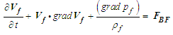 | (1) |
 , with units
  , represents a body force per unit mass that acts on the fluid. Replace term
  with the equivalent vector expression
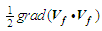
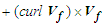 . If we restrict ourselves to body forces that are conservative, we can then replace term
  with the negative gradient of a potential term
  , with units
  , (e.g.,
 for gravity). The Navier-Stokes equation (1) reduces as:
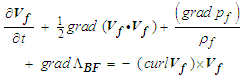 | (2) |
 term is replaced with a barotropic relationship when
  , such that:
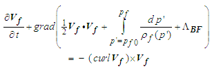 | (3) |
 term (i.e., vorticity) vanishes. However, vorticity will vanish everywhere except along infinitesimally thin vortex lines. In addition, irrotational flow means the velocity vector
  in (3) can be replaced with the gradient of a scalar velocity potential term
  , with units
  , such that:
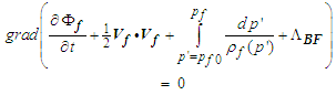 | (4) |
2.3. Bernoulli Function
- The expression within the brackets shown in (4) is called the Bernoulli function
 , with units
  , thus:
 | (5) |
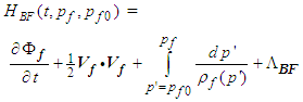 | (6) |
 condition means the Bernoulli function is independent of location along a streamline.Compressibility of a fluid can be defined as the relative change in the local fluid density
  , with units
  , in response to a change in the local fluid pressure
  , with units
  . An adiabatic compression means the entropy content of the fluid remains approximately constant during a compression event. The freestream characteristic speed of the fluid, called the speed of sound
  , with units
  , can be defined [3], such that:
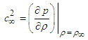 | (7) |
 subscript indicates fluid properties are to be evaluated outside the zone of disturbance.
2.4. Momentum and Continuity Equations
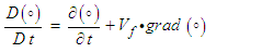
- The momentum equation can be written for a fluid subjected to a conserved body force [4] in terms of a material derivative
 as:
as: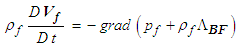 | (8) |
 | (9) |
 in the time interval
  . This change is set equal to the amount of fluid flowing in the volume element minus the amount flowing out of the volume element [3], such that:
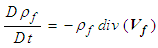 | (10) |
 can be expressed in terms of the fluid velocity for irrotational flow, such that:
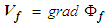 | (11) |
2.5. Compressible, Nonlinear, Convected-Wave Equation
- The momentum and continuity equations can be combined and flow velocity
 replaced with velocity potential
  for irrotational, inviscid, barotropic, isentropic flow [5] [6] subjected to a body force:
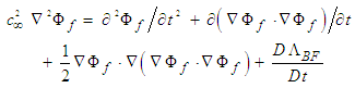 | (12) |
 that is valid for both subsonic and supersonic flow conditions. However, (12) does not hold for transonic velocities since additional terms are needed to account for compression-shock and temperature loses. Replace the velocity potential term
  with a subscript symbol
 , to indicate compressible conditions. One can then write (12) as follows:
 | (13) |
 directed parallel to the positive X-axis. The wave equation (13) is classified as a hyperbolic partial differential equation in terms of spatial coordinate X and time coordinate
  for subsonic speeds.
2.6. Convected-Wave Equation in Cylindrical-Polar Coordinates
- The unsteady convected wave equation (12) can also be written in a cylindrical-polar coordinate system, such that:
 | (14) |
 is the polar radius;
  is the azimuth angle;
  is the Cartesian X-coordinate; and
  is the Cartesian Y-coordinate. The cylindrical-polar velocity components are as follows:
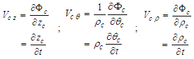 | (15) |
 is the longitudinal velocity component parallel to the longitudinal unit vector
  ; term
  is the circumferential velocity component parallel to the tangential unit vector
  ; and term
  is the radial velocity component parallel to the polar-radial unit vector
  . Hence, one can write the velocity vector for compressible flow conditions
  as the sum of the three vector components:
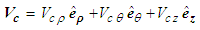 | (16) |
 from (7) is defined as the Mach number for that velocity component, such that:
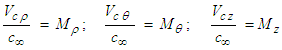 | (17) |
 for a fluid velocity is defined as the sum of its squared components. It must be less than one for subsonic flow conditions:
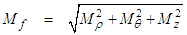 | (18) |
 | (19) |
3. Case 1 - Rotating but Non-Translating Reference frame with a Vanishing Body Force for Subsonic Velocities
- The first case will demonstrate that the 3D nonlinear convected wave equation in cylindrical-polar coordinates for compressible flow conditions with a non-inertial, fixed-to-body reference frame in an unbounded domain reduces to a 2D equation in Cartesian coordinates. This occurs when:1) A source is assumed to consist of a small, slender, solid object;2) Source is fixed to a non-inertial reference frame that rotates at a constant, subsonic, angular speed about the centerline axis;3) Fluid in an unbounded domain is initially at rest;4) Fluids are limited to those that are inviscid (i.e., viscosity
 ), irrotational (i.e.,
  ), barotropic (i.e.,
  ), isentropic (i.e., constant entropy), and compressible;5) No body force acts on the surrounding fluid.Using the above assumptions, we will set the following terms for a rotating but non-translating reference frame and a negligible body force:
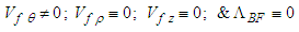 | (20) |
3.1. Linearization of Wave Equation
- The fluid density
 , fluid pressure
  , fluid velocity
  , and velocity potential
  will be linearized as follows with a perturbation component:
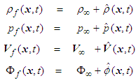 | (21) |
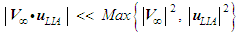
 is used to indicate terms that are evaluated at freestream or undisturbed conditions.It will be assumed that the magnitude of the perturbed velocity
  is much smaller than the magnitude of the freestream velocity
  and that the magnitude of the freestream velocity is much smaller than the characteristic speed of the fluid
  :
: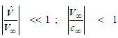 | (22) |
 | (23) |
 , with units
  , is the polar-radius coordinate in the cylindrical-polar coordinate system for compressible flow. All third- and fourth-order perturbation terms have been dropped in (23).
3.2. Change in Variables
- Define the dimensionless parameter
 , spatial variable
  , with units
  , and temporal variable
  , with units
  , for subsonic velocity conditions, where:
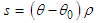 | (24) |
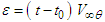 | (25) |
 variable represents an estimate of the circumferential arclength traversed when the azimuth angle changes by the angle
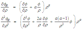
  .Take the following partial derivatives in terms of the
  variable using the chain-rule of differentiation:
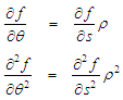 | (26) |
 variable using the chain-rule of differentiation:
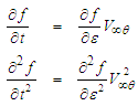 | (27) |
 | (28) |
 and its derivatives, such that
 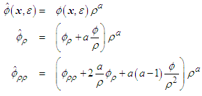 | (29) |
 in (29) is an arbitrary dimensionless coefficient.Replace the potential
  and its derivatives in the wave equation (28) with the new potential
  and divide out the common term
  when finished, such that:
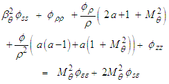 | (30) |
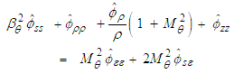
 coefficient equal to
  . The wave equation for a fixed-to-body reference frame (30) simplifies as follows upon back substitution with the new
  coefficient, such that:
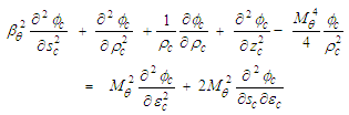 | (31) |
 has been added in (31) to remind us that this equation is based on a compressible fluid assumption.
3.3. Separation-of-Variables
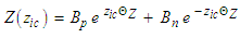
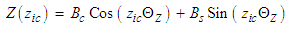
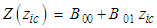
- Consider the following separation-of-variables solution
 , where only the
  component varies with time:
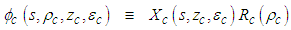 | (32) |
 :
: | (33) |
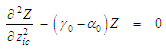
 is an unknown constant coefficient. The
  and
and  terms are independently set equal to
  giving the coupled differential equations:
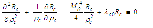 | (34) |
 | (35) |
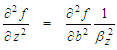
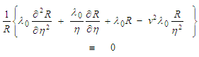
3.4. Wave Equation for the Bessel Laplacian
- The first equation (34), which is not a function of time, is called the wave equation for the Bessel Laplacian. It is of order
 which has non-integer values. The details of the solution will not be presented here but they will be shown in Case 2 to equal:
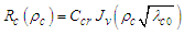 | (36) |
 is an unknown, real valued constant. It should be obvious that the parameter
  must be positive valued for a physically meaningful solution when
  is based on the Bessel function of the first kind
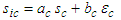
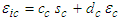
3.5. 2D Wave Equation and Special Relativity
- We will now examine the transient, 2D wave equation given in (35) that includes the term
 . It should be noted that (35) is in the proper form of a 2D Cartesian coordinate system representing a compressible fluid. The coordinate set
  for compressible flow conditions will be transformed to an equivalent coordinate set
  for incompressible flow conditions:
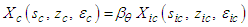 | (37) |
 | (38) |
 | (39) |
 | (40) |
 is defined as
  and
and  are unknown coefficients of the compressible-to-incompressible coordinate transform.The 2D wave equation with term
  can be written in Cartesian coordinates for an incompressible fluid medium with a fixed-to-body reference frame as:
 | (41) |
 | (42) |
 | (43) |
 played no role in the derivation of the transform matrices shown in (42) and (43).All details of the derivations for (42) and (43) can be found in the 2017 [1] paper. Furthermore, [1] shows how the resultant PDE can be converted between sixteen fixed-to-body, fixed-in-space, compressible, and incompressible reference frames.
3.6. Separation-of-Variables: Again
- The wave equation in (41) can be further solved by using the separation-of-variables method a second time by replacing term
 with the following triple product:
 | (44) |
 :
: | (45) |
 since it is independent of the left-hand side expression:
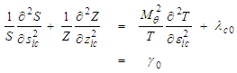 | (46) |
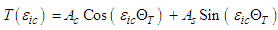
 | (47) |
 and whether the Mach number
  vanishes or not. Three phase angles are defined in terms of the unknown constants:
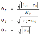 | (48) |
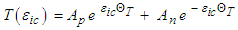
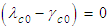
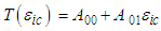
 are as follows:i. If
 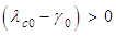 and
and 
 | (49) |
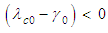 and
and 
 | (50) |
 and
and 
 | (51) |

 | (52) |
 &
&  are unknown constants of integration that are solved based on the boundary conditions in an unbounded domain.Rearrange the left-hand side of equation (46) and solve for the
  component:
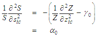 | (53) |
 and solve for
  :
: | (54) |
 :i. If
 | (55) |

 | (56) |

 | (57) |
 are unknown constants of integration that are solved based on the boundary conditions in an unbounded domain.Rearrange the left-hand side of equation (53) and solve for the
  component:
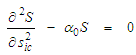 | (58) |
 :i. If
 | (59) |

 | (60) |

 | (61) |
 are unknown constants of integration that are solved based on the boundary conditions in an unbounded domain.
3.7. Final Solution to Case 1
- The final solution of Case 1 for the velocity potential
 of compressible flow in a fixed-to-body reference frame can be written in the following form:
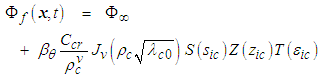 | (62) |
 and
and  to compressible coordinates
  and
and  are listed in (39) and (42). Order
  of the Bessel function is defined as
  .The purpose of presenting Case 1 is to show how the original 3D, nonlinear, convected wave equation (23) in cylindrical-polar coordinates for a compressible fluid in a rotating, but non-translating, fixed-to-body reference frame can be transformed to a system of two partial differential equations. One of the partial differential equation (PDE) expressions is solved as a steady wave equation for the Bessel Laplacian. The other PDE expression is solved as a 2D, transient, wave equation in Cartesian coordinates. This was made possible by converting the azimuth coordinate
  to a circumferential arclength coordinate
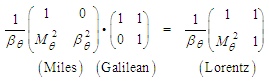
  . It was pointed out in a 2017 paper [1] that the resultant PDE could be converted between sixteen fixed-to-body, fixed-in-space, compressible, and incompressible reference frames. The transformations are based on the Miles, Galilean, and Lorentz matrices.
4. Case 2 - Rotating and Translating Reference Frame Subjected to a Conservative Body Force for Subsonic Velocities
4.1. Introduction to Case 2
- The second case will demonstrate that the 3D nonlinear convected wave equation for compressible flow conditions with a non-inertial, fixed-to-body reference frame in an unbounded domain reduces exactly to the (0+2) focusing cubic NLS equation. This occurs when:1) A source is assumed to consist of a small, slender, solid object;2) Source is a harmonic oscillator of the form
 ;3) Source is fixed to a non-inertial reference frame that rotates at a constant, subsonic, angular speed about the centerline axis;4) Source simultaneously translates at a constant, subsonic speed in a direction parallel to the centerline axis;5) Fluid in an unbounded domain is initially at rest;6) Fluids are limited to those that are inviscid (i.e., viscosity
  ), irrotational (i.e.,
  , except along infinitely thin vortex lines), barotropic (i.e.,
  ), isentropic (i.e., constant entropy), and compressible;7) One or more curved vortex filaments are instantly generated by a source. The filaments remain attached to the source, but they extend into the downwind direction;8) Each curved vortex filament generates an induced velocity in a direction perpendicular to the centerline. The induced velocity produces a conservative body force that acts on the surrounding fluid.
4.2. Wave Equation to be Solved in Case 2
- As previously stated, we shall assume in Case 2 a rotating and translating reference frame subjected to a conservative body force and a harmonic oscillator source:
 | (63) |
 | (64) |
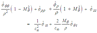
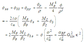
4.3. Linearization of Wave Equation
- The fluid density
 , fluid pressure
  , fluid velocity
  , and velocity potential
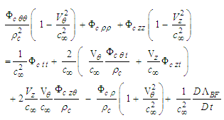
  will be linearized with a perturbation component in the same way as shown in (21) and (22) and substituted into (64). Upon dropping all third and fourth-order perturbation terms, the convected wave equation from (64) reduces to the following:
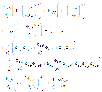
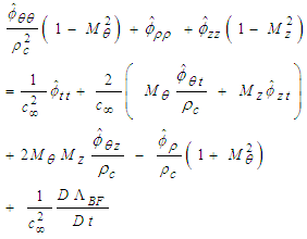 | (65) |
 and
and  are defined in (17).Before proceeding with the solution of (65) for the nonlinear Schrödinger equation, it is worthwhile to review the Madelung transform that has been used since 1927.
4.4. Brief History of Madelung Transforms
- The Madelung transform was first introduced by Madelung [9]. It defines the complex valued wavefunction
 in polar form as
 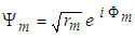 . The argument of the wavefunction equals term
  and the modulus is term
  . The fluid density
  is then identified with term
  and the fluid velocity
  is identified with the gradient operator as
 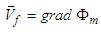 . The Madelung transform only satisfies the (1+1) linear Schrödinger equation. It also brings about an unusual term called the Bohm quantum potential
  that appears in the resultant momentum equation [10], where
 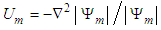 .A more recent and relevant use of the Madelung transformation is given in [10]. He assumes an ideal gas law and temperature
  that is a function of time only. The resultant (1+1) nonlinear Schrödinger equation formulation contains the Bohm-quantum potential
  [11] and the Bialynicki-Birula logarithmic potential [12]. Several exact solutions for inviscid, irrotational, isentropic, and compressible flow are derived [10] but they are essentially restricted to finite domain problems. This is because the velocity and density functions increase indefinitely with distance from the origin.Only the Hasimoto transform [13], in conjunction with LIA based flow theory of curved vortex filaments, is known to be consistent with the (1+1) and (0+2) cubic NLS equations. However, what has completely been absent in the literature is a rational theory demonstrating the derivation or origin of the cubic NLS equation itself using the classical Navier-Stokes equations for compressible flow. This paper will show, apparently for the first time, a derivation based on an aerodynamic application.
4.5. Development of Convected Wave Equation
4.5.1. Source as a Harmonic Oscillator
- The source disturbance will be treated as a harmonic oscillator. The resultant 3D wave will vary harmonically in time. One can then write the perturbed velocity potential
 , with units
  , as a function of a steady-perturbation velocity potential
  , with units
  , and a harmonic component:
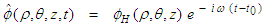 | (66) |
 , with units
  , represents the spin angular speed of the harmonic oscillator source.
4.5.2. Including a New Conservative Body Force
- A conservative body force
 is expressed as the negative gradient of a potential
  :
: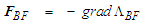 | (67) |
 , with units
  , is related to a potential energy source that is proportional
  , with units
  , to the bending stiffness of an elastic, curved filament vortex undergoing self-induction:
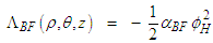 | (68) |
4.5.3. Localized Induction Approximation
- Assuming the applicability of the localized induction approximation (LIA) for a curved filament or vortex, then the velocity induced,
 , with units
  , at position
  along the filament centerline is given by the time derivative of the position vector [13] [14] [15] [16] [17] [18]:
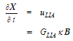 | (69) |
 , with units of
  , is called the coefficient of local induction.
4.5.4. Frenet-Serret Formulas of Differential Geometry
- Term
 in (69), with units of
  , is the curvature of the filament curve and the dimensionless unit vector
  is the binormal vector from the Frenet-Serret formulas of differential geometry [19]. If the dimensionless unit vector
  is the tangent vector parallel to the centerline of the filament curve and dimensionless unit vector
  is the normal vector, then the partial derivative of the tangent vector with respect to arc-length
  along the curve is:
 | (70) |
 is given as [15] [20] [21] [22] [23]:
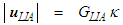 | (71) |
 in (69) and (71) is a function of the vortex strength, radius of the vortex core, and cut-off arclength [13].
4.5.5. Components of the Fluid Velocity Vector 
- At any point in the unbounded domain, the fluid velocity
 will be assumed to consist of freestream velocity
  ; the perturbation velocity
  due to the presence of the solid; slender body moving through the fluid; and the induced velocity component
  generated by the presence of the curved filament
 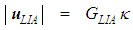 vortex that trails downwind of the slender body that behaves as a harmonic source:
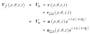 | (72) |
 with units
  is the steady-perturbation velocity component due to the presence of a slender solid body; and
  with units
  is the steady-perturbation velocity component due to the self-inducted velocity produced by the curved filament vortex (i.e., at point
  along the filament).
4.5.6. Gradient of the Steady-Perturbation Velocity Potential
- The gradient of the steady-perturbation velocity potential
 consists of two contributions:
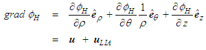 | (73) |
 vanishes if no curved filament vortex forms or if the vortex does not remain attached to the solid, slender translating body.Take the dot product of fluid velocity
  and the
  term from (73):
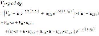 | (74) |
 | (75) |
 | (76) |
 | (77) |
 and
and  given in (74) reduces as follows upon substitution of the assumptions given in (75), (76), and (77):
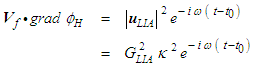 | (78) |
 given in (68) can now be evaluate as follows:
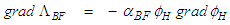 | (79) |
 with the gradient expression given in (78) and (79):
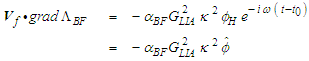 | (80) |
4.5.7. Material Derivative of Body Force Potential
- The time derivative of body force potential
 vanishes since the steady-perturbation velocity potential
  is not a function of time:
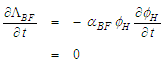 | (81) |
 can now be completely evaluated using the results of (80) and (81)
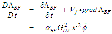 | (82) |
4.5.8. Derivatives of the Perturbed Velocity Potential
- Differentiate the perturbed velocity potential
 from (66) with respect to time for the case when the source is a simple harmonic oscillator with constant amplitude
  and a constant angular speed
  that does not depend on the amplitude:
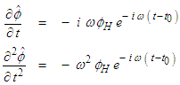 | (83) |
 from (83), the material derivative formula for the body force potential from (82) into the linearized wave equation (65), and divide out the common term
  when finished:
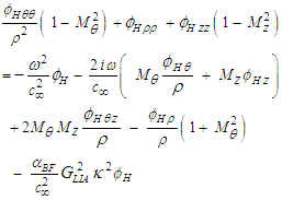 | (84) |
4.5.9. Introducing a New Perturbed Velocity Potential
- Create a new perturbation velocity potential
 , with units
  , to replace the steady-perturbed velocity potential
  , with units
  , where the coefficient
  is unknown:
 | (85) |
 | (86) |
 with term
  and
and  with term
  ; and divide out the common term
  , such that:
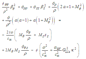 | (87) |
 expression in (87) can be reduced to a standard radial coordinate form by setting coefficient
  equal to the following:
 | (88) |
 from (88) into (87):
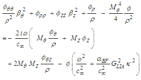 | (89) |
4.5.10. Change in Spatial and Temporal Coordinates
- Define the longitudinal spatial variable
 , with units
  , and the transverse spatial variable
  , with units
  , for subsonic velocity conditions, where:
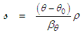 | (90) |
 | (91) |
 variable represents an estimate of the circumferential arclength travelled when the azimuth angle changes by the amount
  and then rescaled by
  The
The  variable represents an estimate of the transvers arclength travelled when the Z coordinate changes by the distance
  and then rescaled by
  Take the following partial derivatives in terms of the
  variable (90) using the chain-rule of differentiation:
 | (92) |
 | (93) |
 variable (91) using the chain-rule of differentiation:
 | (94) |
 | (95) |
 | (96) |
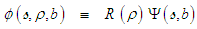
4.6. Separation-of-Variables
- Consider the following separation-of-variables solution
 to the compressible, convected wave equation (96), where only the
  term varies with the polar radius
  :
: | (97) |
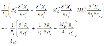
 in (97) is called the wave function of the compressible, convected wave equation given in (96). Substitute the new transform (97) into the wave equation (96) and divide the resultant expression by the term
  :
: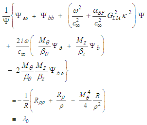 | (98) |
 , with units
  , is an unknown constant.Introduce the following new dimensionless space variable
  to replace the polar radius
  in the
  bracketed expression when the coefficient
  is greater than zero:
 | (99) |
 | (100) |
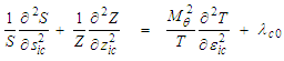
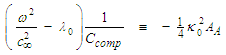
 bracketed expression in (98) after setting it equal to
  :
: | (101) |
 is defined by the following expression:
 | (102) |
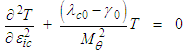
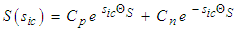
 , such that:
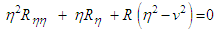 | (103) |
 . It should be obvious from (102) that the order
  is a non-integer with a value always greater than zero for subsonic flow velocities. The general solution to (103) is:
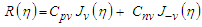 | (104) |
 behave [24] with
 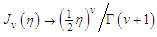 as the argument
  with a fixed value for order
  when
when  ; and where
  is the gamma function. With
  as the argument
  . Bessel functions of the first kind with negative valued orders behave with
  as the argument
  . Hence, the constant
  must vanish for physically meaningful solutions for finite valued induced velocities along the curved filament vortex:
 | (105) |
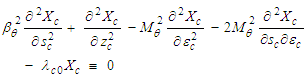
 bracketed expression in (98) that was set equal to
  . Multiply all terms by the wave function
  and rearrange terms, such that:
 | (106) |
4.7. Solving for the Wave Function 
- In the previous section, we solved the separation-of-variable term
 from the convected wave equation as a function of the polar radius. The remaining separation-of-variable term
  , called the wave function, will now be evaluated.
4.7.1. Introducing the Hasimoto transform
- Consider the Hasimoto transform [13], [23], [25] for the complex valued wave function
 when the torsion of the filament vortices is not constant with arclength
  :
: | (107) |
 with units of
  is the torsion of the filament vortex and
  is a reference torsion value. For the special case of constant torsion
  , the Hasimoto transform reduces to the following form:
 | (108) |
 and torsion
  will be considered general functions of arclength
  along the filament and the transverse distance
  from the filament’s centerline.Let
  represent the complex conjugate of the wave function
  , such that from (107):
 | (109) |
 | (110) |
4.7.2. Differential and Riemannian geometry
- The (0+2) NLS equation is formulated in differential geometry using Riemannian geometry with
 and
and  coordinate curves on the
  congruence surface with Riemannian metric [26]:
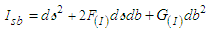 | (111) |
 and
and  are given as
  and
and  on the
  surface. Function
  is called [26] the abnormality of the vector N-field.Two of the constraints for torsion and curvature functions on the
  manifold are called the Da Rios-Betchov equations [25]:
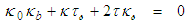 | (112) |
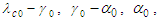
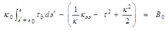 | (113) |
 coefficient is defined as
 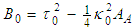 . Terms
  and
and  are integration constants.
4.7.3. Solution for Torsion Function
- A solution for the torsion function
 that satisfies both the LIA assumption, the Hasimoto transform, and Da Rios-Betchov equations on the
  manifold surface is:
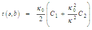 | (114) |
 is defined in terms of LIA based coefficients
  for the filament vortex:
 | (115) |
 are integration and boundary constants.
4.7.4. Conservation Expressions for Torsion, Curvature, and Wave Function
- Differentiate the torsion solution (114) with respect to the
 and then the
  coordinate curves:
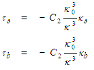 | (116) |
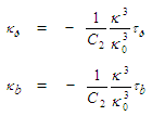 | (117) |
 in (107) with respect to the
  and the
  coordinate curves:
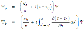 | (118) |
 from (114) and derivative
  from (116) into the first Da Rios-Betchov equation (112) to obtain the conservation expression:
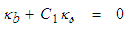 | (119) |
 from (114), derivatives
  and
and  from (117) into the first Da Rios-Betchov equation (112) to obtain the conservation expression:
 | (120) |
 from (119) and
  from (120) into the
  derivative of the Hasimoto transform given in the second line of (118); rearrange and replace the resultant terms using the
  derivative of the Hasimoto transform given in the first line of (118), such that:
 | (121) |
 , torsion
  and wave function
  is apparently new for the (0+2) NLS equation.
4.7.5. Wave Function with Multiple Derivatives
- Differentiate the wave function
 conservation form expression in (121) with respect to the
  and then the
  coordinate curves:
 | (122) |
 from the second line of (122) back into the first line of (122), such that:
 | (123) |
 derivative from (121), the
  derivative from the second line of (122), and the
  derivative from (123) can now be used to replace terms in the (0+2) NLS equation (106), such that:
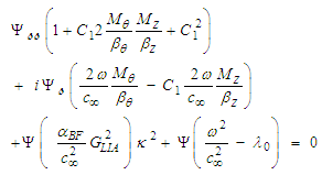 | (124) |
4.7.6. A New Compressibility Constant
- Define a compressibility coefficient
 , such that:
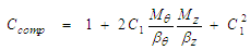 | (125) |
 from the body force term, such that:
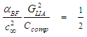 | (126) |
 coefficient from (125) and the
  constant from (126) into the (0+2) NLS equation (124), such that:
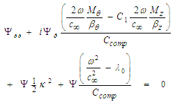 | (127) |
4.7.7. Standard form of the (0+2) NLS
- The standard form of the (0+2) NLS is as follows:
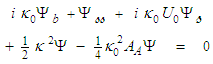 | (128) |
 is called the pseudo-speed coefficient. It is expressed in terms of the reference torsion
  and reference curvature
  values:
 | (129) |
4.7.8. Standard form of the (0+1) NLS
- After eliminating the
 derivative in (128) using the conservation form expression (121), the standard form of the (0+1) NLS is written as follows:
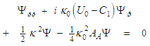 | (130) |
4.7.9. Association of Variables
- Upon comparing the compressible (0+1) NLS in (124) with the standard form of the (0+1) NLS in (130), one can write the following three associations between variables:
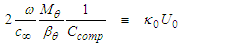 | (131) |
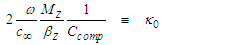 | (132) |
 | (133) |
 from (129) into the first association (131) and solve for the reference torsion
  , such that:
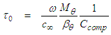 | (134) |
 from the second association (132), such that:
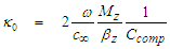 | (135) |
 is evaluated from the third association expression (133), such that:
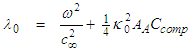 | (136) |
 from expressions (134) and (135), such that:
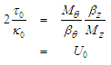 | (137) |
 and separation-of-variables coefficient
  have been expressed in terms of LIA based coefficients
  and aerodynamic source terms
  and
and 
4.8. Solution to the NLS
4.8.1. Differential Equation for Curvature
- Substitute for the derivative
 from the second conservation expression (120) into the integral term in the second Da Rios-Betchov equation (113) and then substitute in the LIA based torsion formula from (114), such that:
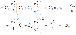 | (138) |
 , such that:
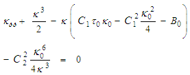 | (139) |
4.8.2. Cubic Polynomial Equation for the Auxiliary Function
- Define the dimensionless auxiliary function
 as
as  . The following cubic polynomial can be obtained by substitution of the auxiliary
  into (139) and integration:
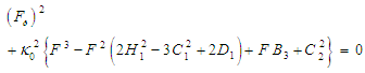 | (140) |
 in (140) is given by:
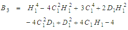 | (141) |
4.8.3. Elliptic function solution for the (0+2) cubic NLS
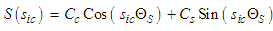
- The solution to the nonlinear ordinary differential equation in (140) is the Jacobian elliptic sine function
 , such that:
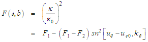 | (142) |
 is the Jacobi modulus; dimensionless term
  is the Jacobian elliptic angle; and
 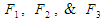 are the three cubic roots when solving the nonlinear ODE given in (140) in terms of the coefficients
  and
and  . Term
  is Kida’s [27] sliding speed coefficient; term
  is a constant of integration for elevation of the resultant vortex filament; and
  is Kida’s [27] translation speed coefficient.An extensive discussion is given in Ch. 6 of [28] for additional constraints imposed on the
  parameters for curve closure, periodicity, and knotting.
4.8.4. Final Solution to Case 2
- The final solution of Case 2 for the velocity potential
 of compressible flow in a fixed-to-body reference frame can be written in the following form:
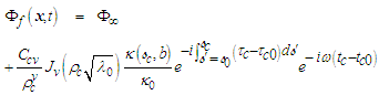 | (143) |
 is listed with coordinates
  and torsion
  to remind us that they are being used under the assumption of a reference frame subjected to compressible flow conditions. Term
  in (143) is given by
  ;
;  is the Bessel function of the first kind, order v;
  is the separation-of-variables integration constant evaluated in (136); arclength coordinate
  is given in (90); transverse arclength coordinate
  is given in (91); torsion function
  is given in (114); curvature function
  is given in (142); reference torsion
  is given in (134); and reference curvature
  is given in (135).
4.9. Summary of Case 2
- Authors since 1927 have solved the logarithmic density version of the (0+1) NLS using the Madelung transform and quantum hydrodynamics. However, a derivation of the (0+1) & (0+2) focusing cubic NLS equation from the Navier-Stokes equation using the Hasimoto transform and an aerodynamic body force is apparently new. The derivation presented here gives the exact expression for the steady form of the cubic NLS that matches the curvature and torsion constraints derived from Riemann geometry for curved surfaces.Case 2 involves the transient, 3D, nonlinear, convected wave equation (64) in a fixed-to-body reference frame for a compressible fluid with constant coefficients expressed in cylindrical-polar coordinates for a source that is both rotating and translating. There are three reasons for presenting this problem: the first is to show that the (0+2) cubic NLS is embedded within the PDE of the original wave equation (after converting the partial derivatives
 and
and  ); the second is to show that the (0+1) cubic NLS is embedded within the PDE of the wave equation; and the third is to show that there is an analytically solution (143) to the wave equation (64). The conversion of the partial derivates
  ,
,  , and
, and  is based on the discovery of three new conservation form expressions (119), (120), & (121) for the curvature
  , torsion
  and wave function
  .
.5. Discussion
- This article examines the derivation and solution of unsteady convected waves for compressible fluids using an analogous problem from aerodynamics. The take-away conclusion is that one is able to scale from the smallest-to-largest and slowest-to-fastest processes in the universe using Newton’s classical laws for fluids based on a system of absolute space and time coordinates. This is made possible by recognizing and retaining the effects of fluid compressibility that are intrinsically associated with the cross-derivative terms between space and time. The retention of the cross-derivatives makes the resultant convected nonlinear wave equations more difficult to solve. In compensation, it eliminates the artificial contradictions and mysticisms imposed with using elastic space-time coordinates when one insists on assuming incompressible flow conditions for in vacuo problems.This paper and the 2017 paper [1] don’t reject the scientific data obtained from 100 years of testing special relativity. What is presented here is a radically different physical interpretation of prior test results. Instead of interpreting the special relativity tests as proof-of-errors in ignoring the elasticity of relative space-time coordinates, it interprets prior tests as showing the error in dropping the nonlinear cross-derivatives from the convected wave equation that uses an absolute space and time coordinate system.It might seem to be argumentative to reject the classical understanding on why speed affects the measurement of distance but it actual goes to the heart of science: progress is made by challenging theories that one takes for granted and replacing it with an improved version, with each iteration bringing humanity closer to the truth. The unmasking of the cubic NLS and special relativity relationships within the compressible, convected wave equation for laminar flow offers proof in the value of challenging what one thought was totally understood for more than a century.
6. Conclusions
- For the first time, an exact derivation of the (0+2) cubic NLS equation is obtained after combining the 3D Navier-Stokes equation, the Hasimoto transform, and an aerodynamic body force for induced velocity. Authors have previously derived a special logarithmic density version of the NLS using the Madelung transform and quantum hydrodynamics. However, the derivation given here results in an exact expression for the steady form of the (0+2) cubic NLS that matches the curvature and torsion constraints derived from Riemann geometry for curved surfaces. In addition, it is shown how special relativity expressions are obtainable within the steady-rotating source problem of the convected wave equation when written in cylindrical-polar coordinates and a non-inertial fixed-to-body reference frame.
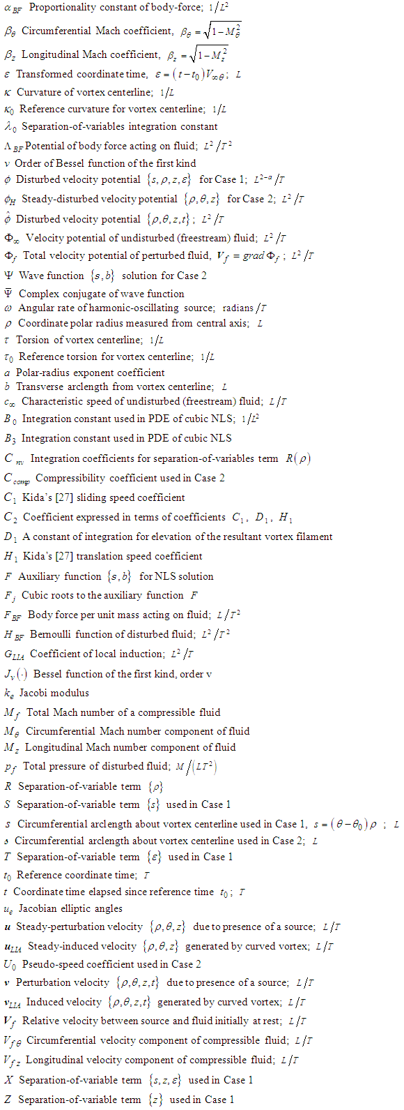
Nomenclature