Doron Kwiat
17/2 Erez Street, Mazkeret Batyia, Israel
Correspondence to: Doron Kwiat , 17/2 Erez Street, Mazkeret Batyia, Israel.
| Email: |  |
Copyright © 2018 The Author(s). Published by Scientific & Academic Publishing.
This work is licensed under the Creative Commons Attribution International License (CC BY).
http://creativecommons.org/licenses/by/4.0/

Abstract
One can represent quantum mechanics with real wave functions. The use of real wave functions leads to the interpretation of a single particle as consisting of two entities represented as coupled wave functions. Probability distributions are shown to be preserved for coupled wave functions just as for a single complex function. Assuming a string model [12-17], a double coupled string description is suggested, whereby the Schrödinger equation emerges naturally. This double-string description assumes a time-dependent tension [18] in the strings, together with a time-dependent interaction between the two strings. If the time pattern is similar for both tension and interaction, their ratio is shown to be ℏ/2. This leads to the derivation of Planck's constant as a result of strings interactions and characteristics.
Keywords:
Quantum Mechanics, Strings, Planck Constant
Cite this paper: Doron Kwiat , The Schrödinger Equation and Asymptotic Strings, International Journal of Theoretical and Mathematical Physics, Vol. 8 No. 3, 2018, pp. 71-77. doi: 10.5923/j.ijtmp.20180803.03.
1. Introduction
The Schrödinger equation is a mathematical equation that describes changes over time of a physical system in which quantum effects, such as wave–particle duality, are significant. These systems are referred to as quantum (mechanical) systems. The equation is considered a central result in the study of quantum systems, and its derivation was a significant landmark in the development of the theory of quantum mechanics. It was named after Erwin Schrödinger, who derived the equation in 1925 and published it in 1926 [1].In 1952, Bohm [2] attempted to justify the Schrödinger equation with the existence of hidden variables. In 1966, Nelson [3] suggested a classical formulation of the equation, based on the hypothesis that every particle of mass m is subject to a Brownian motion with a diffusion coefficient ℏ/2m and no friction. Ever since, many solutions have been given to the Schrödinger equation, for various physical systems [4-10]. In this work, a formulation of quantum mechanics without use of complex numbers is described and is shown to be equivalent to the complex formulation. Moreover, dealing with the real and imaginary parts separately, a single particle shows a 2-entities behavior. As a result, a double-string description is suggested, whereby the Schrödinger equation emerges naturally. This double-string description assumes a time-dependent decaying tension in the strings, together with a time-dependent interaction between the two strings. If the decay pattern is similar for both tension and interaction, their ratio is shown to be ℏ/2.
2. A Non-relativistic Schrödinger Equation
In non-relativistic quantum mechanics, a particle (such as an electron or proton) is described by a complex wave-function, ψ(x, t), whose time evolution is governed by the Schrödinger equation [9]: | (1) |
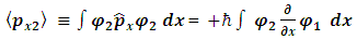
Here, m is the particle's mass and V(x) is the applied potential. Physical information about the behavior of the particle is extracted from the wave function by constructing expected values for various quantities; for example, the expected value of the particle's position is given by integrating ψ*(x) x ψ(x) over all of space, and the expected value of the particle's momentum is found by integrating −iħ ψ*(x) ∂ψ/∂x. The quantity ψ*(x)ψ(x) is itself interpreted as a probability density function. This treatment of quantum mechanics, where a particle's wave function evolves against a classical background potential V(x), is sometimes called first quantization.  may be written as a linear combination of the functions
  , which are solutions of
  .
.  may be interpreted as the probability density of a single particle in the ith energy state, to be found at an interval dx around position x.
3. Real Wave Functions
The introduction of imaginary and complex numbers is nothing but a mathematical convenience for shortening and unifying our equations. Physical problems cannot rely on imaginary numbers, except for the purpose of mathematical comfort. Obviously, since complex entities can always be decomposed into real and imaginary parts and vice versa, using natural (real-entities only) approach does not contribute anything and makes things unjustifiably more complex. But, by using complex presentation we might be overlooking some hidden qualities.The basic equation of quantum mechanics is the famous one-particle time-dependent Schrödinger equation: | (2) |
where i is the imaginary number  is the reduced Planck constant which is
  , the symbol ∂/∂t indicates a partial derivative with respect to time t,
  (the Greek letter psi) is the wave function of the quantum system, x is the position in a one-dimensional coordinate system, and t the time.
  is the Hamiltonian operator (which characterizes the total energy of the system under consideration).Where
 | (3) |
with  and where
  is the potential energy, which may also have real and imaginary parts
  and
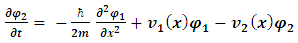
and  , respectively.As described by Hatfield [16], One may separate the complex wave function into its real and imaginary components.
 | (4) |
Using a vector notation may be useful: | (5) |
and the Schrödinger equation may be written: | (6) |
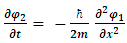
or When separated into real and imaginary components, it is equivalent to:
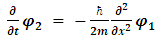
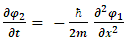
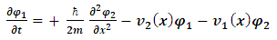 | (7) |
 | (8) |
This form indicates the coupling that exists between the two constituent entities, which comprise the "single" particle.We remember that  is interpreted as the probability density of finding a single particle at an interval dx around position x.Likewise, since
 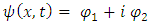 and
and 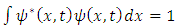 then
then | (9) |
Here, all integrals over f(x) are definite integrals over an interval of length 
 | (10) |
Therefore, one may interpret this as two particles interacting with each other, whose probability densities  and
and  are affected by each other, and yet, they sum up to 1. However, we cannot tell their probabilities apart.The Schrödinger equation is now interpreted as two probability density functions coupled according to eqs. [7] and [8].The complex wave equation of a single particle, as described by the Schrödinger equation, is actually a mathematical description of two real wave functions. A single particle may be interpreted as a coupled two-waves entity (particles?).Surprising ResultsPresentation of quantum mechanics with real wave-functions does not produce contradicting results to the complex presentation. This is obvious, as complex presentation is nothing but a mathematical manipulation of real variables.However, when using real wave functions, some hidden characteristics emerge.We shall see in the following, that the two real entities of which the particle comprises of, behave in an unexpected manner.
4. Linear Momentum
In terms of quantum mechanics, we have for the particle's momentum: | (11) |
Looking at the real and imaginary parts separately, we see that this is equivalent to: | (12) |
 | (13) |
Using equations [7, 8], the Schrödinger equation for a free particle (v(x) =0) is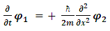 | (14) |
 | (15) |
Multiply eq [14] and [15] by  and
and  respectively, one obtains:
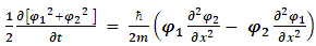 | (16) |
Integrate over x, on the l.h.s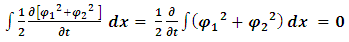 | (17) |
Therefore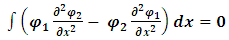 | (18) |
Also,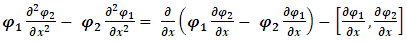 | (19) |
and since 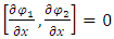 we obtain:
 | (20) |
Hence, combining this with the result in [18] gives: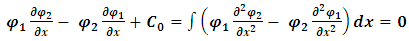 | (21) |
and therefore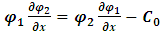 | (22) |
(unless we put the integration limits at ±L/2, we cannot omit the integration constant).If 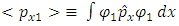 represents the observable momentum px1 and
 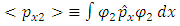 represents the observable momentum px2, we obtain:
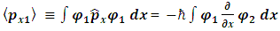 | (23) |
 | (24) |
Summing equations [23] and [24], and using [22] results in: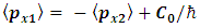 | (25) |
The total momentum is: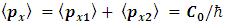 | (26) |
And if we designate the total momentum by p, then  For zero total momentum,
  , we see that
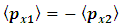 | (27) |
Meaning that the two entities have opposite linear momentum.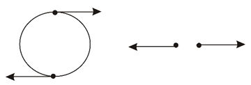 | Figure 1. A combined particle of two opposite momenta, with either linear or circular motion |
This can be resolved if the two constituents are spinning in opposite directions around a common center, or if the two components are entangled and moving linearly away in opposite directions. But the latter solution will not allow us to observe them in one place simultaneously.
5. Angular Momentum
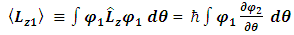
Assuming spherical symmetry, with polar angle  , the z-component of its angular momentum in spherical coordinates is
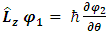
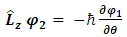
  .To find the eigenvalues we write:
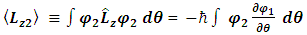
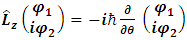 | (28) |
 | (29) |
 | (30) |
Suppose m1, m2, are the angular momentum eigenvalues for each entity of the particle: | (31) |
 | (32) |
 | (33) |
 | (34) |
Equations [34] and [35] can be immediately solved to give: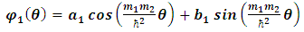 | (35) |
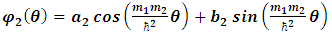 | (36) |
Assuming a boundary condition 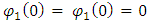 We find
  | (37) |
And therefore | (38) |
And therefore 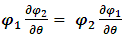 | (39) |
 | (40) |
 | (41) |
We conclude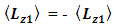 | (42) |
Thus, independently of the composite spin for this particle, its two components (entities) will have an opposite spin.
6. A 2-string Analog to the Schrödinger Equation
Assume a one-dimensional description in x, and time t.Let a single particle of mass m be described as consisting of two classical real strings,  and
and  . Here, the functions,
  and
and  represent the amplitudes of the perturbation of the strings from the x-axis as a function of time and position.Let the coupling between these two strings be given a constant Ks and described by the following coupled, differential equations:
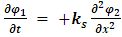 | (43) |
 | (44) |
Let us present a physical consideration of these two equations.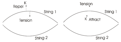 | Figure 2. Closed-loop double-strings. Attraction, or repulsion and tension, will change directions according to the deviation from the steady-state |
Consider two strings  and
and  . Let
. Let  represent the displacement in the string at time t and position x. Let
  be the tension in the string. Though we start in a classical model, this can be directed to modern string models too [18]. It is well known that the force exerted by this tension on a string element X (see figure 3) is described by:
 | (45) |
Suppose now that this string is connected by an endless number of springs to a second string, which is described by  . Let the individual springs each have a spring constant Ks. Assume further that this spring constant is not fixed in time. Rather, it changes with time, starting at time t0, the moment in which the two strings interact. Suppose the two strings are bound together at their ends, thus creating a closed loop. Suppose further that the closed loop of strings is at an equilibrium state. The tension in both strings is assumed to be changing in time. There is an interaction force exerted between the strings, pushing them apart or towards each other, against the tendency to collapse or to expand due to tension forces. This will happen when, for some reason, the two strings are perturbed from their steady-state equilibrium of tension and distance.
 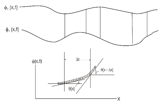 | Figure 3. A double-string analog, as described in Eqs. [43, 44]. The angleθ describes the tangent, in the approximation of tanθ ≈ sinθ for θ << 1 |
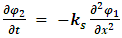
As the force tends to weaken or strengthen the interaction as it stretches apart or contracts from its steady state, it is therefore reasonable to assume that the sprig constant changes as: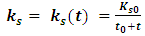 | (46) |
We may then assume that the tension force in string 1 creates a disturbance from equilibrium  in string 2, proportional to the spring constant Ks and to the string mass
  .Since
  describes a displacement amplitude, it has the dimensions of [m].The force in Eq [45] has dimensions [kg][m]/[sec2].We may then write
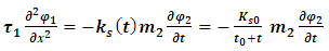 | (47) |
Notice, that Ks0 is dimensionless (or, has dimensions set according to the dimension of  ).Rearranging [4] we obtain:
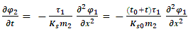 | (48) |
By the same argument,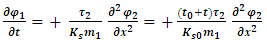 | (49) |
For reasons of symmetry we assume 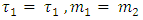 Furthermore, we will assume also that the string tension
  , decays with time in the same manner as the interaction spring force
  .Thus,
 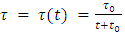 The resulting two equations for the interacting strings are now:
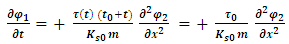 | (50) |
 | (51) |
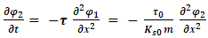
The resulting two equations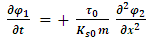 | (52) |
 | (53) |
are similar to the coupled wave functions equations: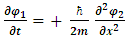 | (54) |
 | (55) |
provided that | (56) |
This relates the initial tension  in the strings to the initial coupling
  between the two strings. As
  and Ks are inversely proportional to time, the ratio
  is fixed in time. This interpretation of a particle as consisting of two coupled strings whose tensions and interaction are inversely proportional to time gives us a classic interpretation of the Schrödinger equation.This relates the initial tension
  in the strings to the initial coupling
  between the two strings. As
  and Ks are inversely proportional to time, the ratio
  is constant in time.We will assume now, without loss of generality
 | (57) |
7. Asymptotic Correction
Since the denominators’ ratio cancels out, the  ratio remains constant in time, however each of them decays to 0 as
  .In order to avoid the vanishing of tension and the mutual spring interaction, we may introduce a different time dependency:
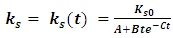 | (58) |
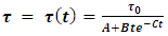 | (59) |
With A, a constant of dimension [sec].The time behavior is now different, but the ratio  remains constant in time as before. But now, the vanishing of the constants as
  is avoided. We also notice that for both
  and K the parameters A, B, and C must be the same, otherwise the ratio will become time dependent.Characteristics of the interactionDefine the function f(t):
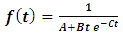 | (60) |
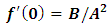
By investigating its behavior, we see that f(t) is bounded and has a minimum at some tmin. After this minimum, it returns asymptotically to its initial value.The upper bound on f(t) is given by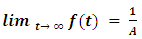 | (61) |
The minimum is obtained at  , and at minimum
 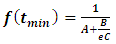 | (62) |
And the following is also true: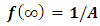 | (63) |
 | (64) |
and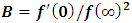 | (65) |
This may be interpreted as a double string initially at a steady state, with a constant tension  . Then, for some reason, an interaction (disturbance) occurs and the tension drops to minimum at time tmin = 1/c and then gradually returns to its initial steady-state tension
  (0). A similar argument is true for the interaction constant K.
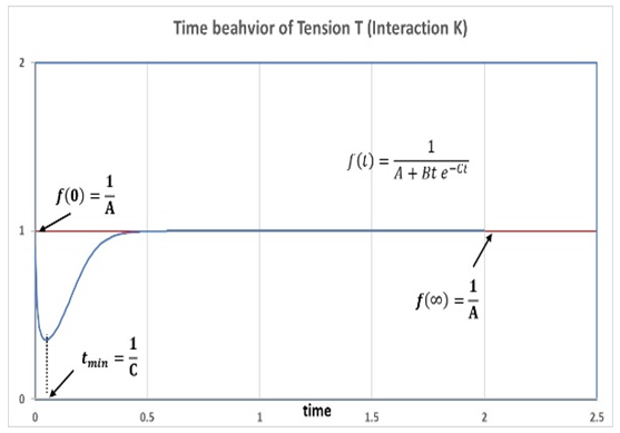 | Figure 4. Time behavior of tension τ in a string and interaction constant K between two strings. Behavior is governed by the function f(t) given in Eq [60]. Parameter A controls the level of stable-state equilibrium given by 1/A. The amplitude drops for a while and rises back to equilibrium, with minimum obtained at time tmin = 1/C. (This figure used A=1, B=100, c= 20) |
This describes a single particle of mass m, whose interaction parameters at time t < t0 are null: B= C=0.At time t0 an interaction occurs, whose intensity energy Ei may be estimated by f(tmin)2 or in other words: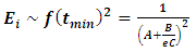 | (66) |
We see that the particle has a fixed amplitude for its component strings until the time of perturbation (collision?). The perturbation energy Ei creates a temporary displacement of amplitudes in the strings, which asymptotically return to their original equilibrium steady-state.Complex wave-functionsEquations [54], [55] then give: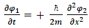 | (67) |
 | (68) |
Defining the complex function 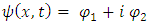 Eqs [67] and [68] may be combined together:
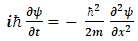 | (69) |
By multiplying [67] and [68] by  and
and  respectively, integrating over x, and imposing the mixed boundary conditions ∂/∂x, = 0 on both functions at L → ± ∞, it is immediately shown that (up to a normalization factor):
 | (70) |
Hence,  | (71) |
Thus, the classic coupled string system may be interpreted as a quantum mechanical single particle, described by a wave function  which is a probability distribution function. This function describes a free particle of momentum
 | (72) |
When substituted in 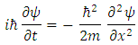 The result is
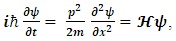 | (73) |
A free particle Hamiltonian.
8. Interpretation
This interpretation of a particle as made up of two real coupled strings whose tensions and interaction are inversely proportional to time is equivalent to the single-particle complex wave function described by the Schrödinger equation. When the original Schrödinger equation is used with a complex wave function, this internal string-like characteristic is not apparent because we treat the real and imaginary parts as a single entity. However, when the equation is separated into two parts, these two parts can be treated as independent strings interacting with each other, where both tension and interaction fall off abruptly and inversely proportional to time. This may be a result of weakening due to increased distance between the two strings, together with a drop in tension inside the strings.Since each of the wave functions is now a real function of time and position, and since the sum of the squares of the two wave functions equals 1 (Eq [70]), these wave functions can describe the actual strings on one hand and be interpreted as probability distribution functions on the other hand. This unifies the two interpretations into one: A single-particle quantum mechanical description with a single complex wave function, which is equivalent to a classic description of two interacting strings. The quantum quality emerges when we understand that the ratio between the string tension and the interaction constant are time dependent and the ratio is constant in time, namely the Planck universal constant,  .When the original Schrödinger equation is used with a complex wave function, this internal string-like characteristic is not apparent because we treat the real and imaginary parts as a single entity. However, when the equation is separated into two parts, these two parts can be treated as independent strings interacting with each other where both tension and interaction fall off abruptly inversely proportional to time. This may be a result of weakening due to increased distance between the two strings, together with tension drop inside the strings.The result is the familiar Schrödinger equation.
9. Connection of Strings Structure to Gravity
Tension  and the Planck constant
  , may be connected with the
  (alpha prime) parameter [19] and the gravitational constant G.Particles in a string theory are like the harmonic notes played on a string with a fixed tension
 The parameter
  is called the string parameter and the square root of this number represents the approximate distance scale at which string effects should become observable.Since
  , and as the minimum observable length for a quantum string theory is given by
 | (74) |
then, if string theory is a theory of quantum gravity, this minimum length scale should be at least the size of the Planck length. Since it is the length scale made by the combination of Newton's gravitational constant G , the speed of light c and Planck's constant, 
 | (75) |
Thus | (76) |
This indicates to the connection between the structure of the string structure to the three known constants of nature.Expanding to other particlesIf we accept the claim that a single, non-relativistic Schrödinger equation is a description of a single massive particle made up of two coupled strings, then we may project from this to the relativistic Dirac equation: | (77) |
Instead of a 4-spinor solution we may assume an 8-string solution, with each spinor made up of 2 coupled strings. To do this we separate the complex wave function  into its real and imaginary parts, and by using them in the Dirac equation we will obtain two separate equations where the imaginary and real parts are separated. This same procedure can be applied to any quantum field Lagrangian, resulting in the doubling of the number of equations on one hand, but gaining a separation of the equations into real wave functions on the other. These wave functions may be interpreted as coupled strings.
10. A Balloon Model
In a 3D version, we can illustrate our concept with a balloon version. The spherical balloon has an internal pressure P that tends to inflate the balloon by exerting force perpendicular to the surface area. The surface area of the balloon has an internal tension force τ acting in the opposite direction, also perpendicular to the surface area, but opposing the force of internal pressure.At equilibrium, the forces of inward tension and outward pressure are equal.If at a given instance t0, a small disturbance occurs that moves the surface off its equilibrium, the force of tension will increase along with the pressure, which will bring the surface back to equilibrium. If, on the other hand, the balloon surface is pushed outwards, the pressure will decrease and the tension will increase in the opposite direction.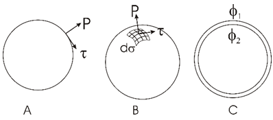 | Figure 5. A closed string with "pressure" P and tension τ (A) and a 2-dimensional surface area of a balloon-like string, with forces acting on an infinitesimal area dσ (B). For our model, we may assume two separate, closely packed and interacting (coupled) balloons (C), denoted by  |
Pressure force P and tension force τ are always perpendicular to the surface area and in opposite directions. Both P and τ will change in time due to some unsettling interaction. In its steady state, the balloon may be expanding or contracting at a steady rate but the ratio τ/P must be kept constant.Instead of a coupled strings model, we may assume double sphere-like surfaces, one enclosed inside the other, with a very small gap between the two. Both have surface tension τ and they interact with each other with an interaction force K.
11. Conclusions
One can do quantum mechanics with real wave functions instead of complex ones.Using real wave functions leads to the interpretation of a single particle as consisting of two interacting entities. This coupled-strings interaction model leads to the Schrödinger equation for a single particle. Assuming Tension τ in a string and interaction force K between strings are time dependent, then the ratio τ/K asymptotically equals Planck's constant  . This gives us a derivation of Planck's constant out of fundamental interaction physical model. Even though these interactions may become perturbed by some external interactions, it is shown here that these sudden perturbations affect the coupling only temporarily, and the system of coupled strings returns asymptotically to a steady-state equilibrium.A single particle may consist of coupled 2D spherical sheets (membranes) of a given surface tension and mutual interaction force; both are time dependent and asymptotically return to equilibrium.
References
| [1] | Erwin Schrödinger, An Undulatory Theory of the Mechanics of Atoms and Molecules. Physical Review. 28 (6): 1049–1070. 1926. |
| [2] | David Bohm, A Suggested Interpretation of the Quantum Theory in Terms of "Hidden" Variables. I, Phys. Rev. 85, 166 – Published 15 January 1952. |
| [3] | Edward Nelson, Derivation of the Schrödinger Equation from Newtonian Mechanics, Phys. Rev. 150, 1079 – Published 28 October 1966. |
| [4] | M.D Feit J.A FleckJr. A Steiger, Solution of the Schrödinger equation by a spectral method. Journal of Computational Physics, Volume 47, Issue 3, September 1982, Pages 412-433. |
| [5] | D Kosloff R Kosloff, A Fourier method solution for the time dependent Schrödinger equation as a tool in molecular dynamics, Journal of Computational Physics, Volume 52, Issue 1, October 1983, Pages 35-53. |
| [6] | Peng Zhang, Y. Y. Lau. Ultrafast strong-field photoelectron emission from biased metal surfaces: exact solution to time-dependent Schrödinger Equation, Scientific Reports volume 6, Article number: 19894 2016. |
| [7] | A. Berezin, L. D. Fadeev A remark on Schrödinger's equation with a singular potential, Fifty Years of Mathematical Physics, Part 3. Field Theory: pp. 133-135, 2016. |
| [8] | Cheemaa N, Younis M, New and more general traveling wave solutions for nonlinear Schrödinger equation. Journal of Waves in Random and Complex Media, pp 30-41, Volume 26, 2016 - Issue 1. |
| [9] | Pavel Kundrát and Miloš Lokajíček. Three-dimensional harmonic oscillator and time evolution in quantum mechanics. Phys. Rev. A 67, 012104 –13 January 2003. |
| [10] | Milos V. Lokajíček, Schroedinger equation and classical physics. |
| [11] | Jon H. Shirley Solution of the Schrödinger Equation with a Hamiltonian Periodic in Time, Phys. Rev. 138, B979 – Published 24 May 1965. |
| [12] | Leonard Susskind, Art Friedman, "Quantum Mechanics: The Theoretical Minimum", Penguin, Published 30th April 2015. |
| [13] | Leonard Susskind Structure of Hadrons Implied by Duality, Phys. Rev. D 1, 1182, 1970. |
| [14] | Y. Nambu, Strings, monopoles, and gauge fields, Phys. Rev. D 10, 4262.1974. |
| [15] | H.B. Nielsen, P. Olesen, Vortex-line models for dual strings, Nuclear Physics B, Volume 61, 24 pp 45-611973. |
| [16] | Brian Hatfield, Quantum Field Theory of Point Particles and Strings. Mathematical Physics Research, CRC Press, 2018, Taylor & Francis Group. |
| [17] | Grassi, A., Hatsuda, Y. and Mariño, M., Topological Strings from Quantum Mechanics, Ann. Henri Poincaré 2016 17: 3177. https://doi.org/10.1007/s00023-016-0479-4. |
| [18] | A.Polyakov, Fine structure of strings, Nuclear Physics B. Volume 268, Issue 2, 1986, pp 406-412. |
| [19] | J. Louis, T. Mohaupt, and S. Theisen, String Theory: An Overview, Max Planck Institute for theoretical Physics, http://www.aei.mpg.de/~theisen/LMT.pdf. |

 Abstract
 Reference
 Full-Text PDF
 Full-text HTML