-
Paper Information
- Previous Paper
- Paper Submission
-
Journal Information
- About This Journal
- Editorial Board
- Current Issue
- Archive
- Author Guidelines
- Contact Us
International Journal of Theoretical and Mathematical Physics
p-ISSN: 2167-6844 e-ISSN: 2167-6852
2017; 7(5): 113-131
doi:10.5923/j.ijtmp.20170705.02

Deriving Special Relativity from the Theory of Subsonic Compressible Aerodynamics
 Abstract
 Reference
 Full-Text PDF
 Full-text HTML
Michael James Ungs
Tetra Tech, Lafayette, USA
Correspondence to: Michael James Ungs, Tetra Tech, Lafayette, USA.
| Email: |  |
Copyright © 2017 Scientific & Academic Publishing. All Rights Reserved.
This work is licensed under the Creative Commons Attribution International License (CC BY).
http://creativecommons.org/licenses/by/4.0/

Mathematical transformations that convert the convected wave equation in subsonic compressible flow to one based on incompressible flow have profound implications in understanding the physical basis of the transformations used in the theory of special relativity. The evolution of using incompressible flow solutions for airfoil design in lieu of conducting high speed wind tunnel tests is briefly reviewed. This in turn evokes the forgotten history of aerodynamicists using the Prandtl-Glauert method of spatial contraction as a substitute for compressibility effects before WWII. Matrix expressions identical in form to those representing relativistic velocity, acceleration, and mass are developed from linear transformations relating compressible versus incompressible flow systems and fixed-to-vehicle versus fixed-in-space coordinate reference frames. The mathematical intersection of special relativity and compressible flow theory is generally not understood nor appreciated outside the field of subsonic aerodynamics, making it a compelling subject for us to explore.
Keywords: Compressible flow, Convected wave equation, Incompressible flow, Lorentz factor, Prandtl-Glauert factor, Special relativity
Cite this paper: Michael James Ungs, Deriving Special Relativity from the Theory of Subsonic Compressible Aerodynamics, International Journal of Theoretical and Mathematical Physics, Vol. 7 No. 5, 2017, pp. 113-131. doi: 10.5923/j.ijtmp.20170705.02.
Article Outline
1. Introduction
- The development of a comprehensive theory of flight has been a slow, frustrating study in progress. An interesting account of its complex history up to the 1930s in Europe is given by [1]. Briefly stated, the question of interest revolves around using the approximate, ideal fluid theories of Bernoulli and Euler versus using the more exact, non-linear Navier-Stokes equations. By the beginning of the 1940’s, a lot of low speed data had been collected from wind tunnel testing of standardized airfoil sections for subsonic aerodynamic research by the National Advisory Committee for Aeronautics [2, 3]. Using incompressible flow theory, the wind tunnel data were processed and formulated into tables and graphs suitable for aircraft development and design. The near universal assumption of incompressible flow for manned flight was quite reasonable at that time considering air speeds less than 200 miles per hour were typically involved, with only the tips of high speed propellers approaching the speed of sound. With the development of faster planes and jets, such as the 500 mph Messerschmitt Me262, it became imperative that methods be devised that would allow the older low speed, incompressible based tabulations to be used with simple correction factors so that the effect of compressibility could be accounted for when designing aircraft for higher speeds. The alternative was to build faster wind tunnels and to painstakingly redo the airfoil tests and tabulations.Analytical methods to compensate incompressible based lift calculations are called compressibility corrections. The Prandtl-Glauert method is one such approach that assumes two-dimensional, incompressible flow parallel to an airfoil cross section and then reduces the length of the airfoil chord in the lift and moment equations to account for compressibility [4]. The effect of mathematically compressing the parallel axis coordinate can be easily accounted for in two dimensions. However, in three dimensions, stretching and compressing the parallel axis coordinate results in lateral coordinate effects that produce non-linear changes in wing forces and moments [5, 6]. To the aeronautical engineer, contracting chord length and other aircraft dimensions as a function of speed in expressions formulated on the basis of incompressible flow is not controversial. It will be shown that these spatial contractions are mathematical artefacts induced while performing transformations from one coordinate system to another.Interest expressed by the aeronautical community in using coordinate transformation methods to convert incompressible to compressible flow has substantially decreased since the 1950s. It has been replaced with methods that directly solve the fluid dynamic equations of compressible flow using fast computers and software based on computational fluid dynamics. None the less, there is still interest in special applications such as for steady-state flow problems. Examples of this are seen by the use of a power series expansions in terms of the Mach number [7] and using a variable density and flow angle for mapping in two dimensions [8].A link between special relativity and compressible fluid dynamics is not a new concept [9, 10]. But it is rarely pursued outside the shadow of unconventional physics. The purpose of this article is to systematic examine the mappings between compressible and incompressible flow systems in different coordinate frames and to show the profound similarity between special relativity and the convective wave equation expressions.We shall assume air is a continuous fluid with fluid properties that are irrotational, inviscid, barotropic, and isentropic. There are also two flow systems considered that affect the form of the wave equation when solving for the perturbation velocity potential. In both cases, the X-axis of the coordinate system is aligned with the direction of the free-stream velocity vector. The x=0 coordinate is located at the airfoil’s leading edge and coordinate values increase towards the trailing edge. Compressible flow refers to the representation of the wave equation for the perturbation velocity potential in which there are cross-derivative terms between the X, Y, Z spatial coordinates and the time coordinate. Incompressible flow is defined as flow within which the fluid density remains constant with pressure. It is represented with a wave equation for the perturbation velocity potential in which there are no cross-derivative terms. These two flow systems are linked by coordinate transformations.Two reference frames are also considered. There is the non-inertial, fixed-to-vehicle (FTV) reference frame with coordinates attached to the leading edge of the vehicle. The vehicle remains at rest as the fluid medium flows against the leading edge with free-stream velocity
 , where
 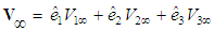 . The other is the inertial, fixed-in-space (FIS) reference frame with the fluid medium initially at rest and the vehicle moving with speed
2. Convected Wave Equation
2.1. Transient Case
- Consider the fluid dynamics of a moving fluid medium that is compressible. The adiabatic compression of a fluid
 can be defined as the relative change in the local fluid density
  and adiabatic compressibility coefficient
  in response to a change in the local fluid pressure
  , such that
  . In addition, the free-stream squared-speed of sound
  is inversely proportional to the adiabatic compression
  evaluated at the free-stream fluid density
  , such that:
 | (1) |
 | (2) |
 is written out as the sum of two contributions, where
  is a tensor derivative of the fluid velocity
  :
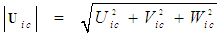
: | (3) |
 is defined as the fluid velocity
  for a stationary medium. However, when the medium is also moving with a free-stream velocity
  , then the free-stream contribution can be separated from the perturbation velocity component
  , such that
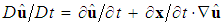
 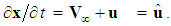 The convective form of the continuity equation for the conservation of mass can be expressed in terms of the divergence of the fluid velocity, such that:
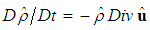 | (4) |
 can be expressed in terms of the fluid velocity for irrotational flow, such that:
 | (5) |
 | (6) |
 ), inviscid (i.e.,
  ), barotropic (i.e.,
  ), isentropic (i.e., constant entropy) flow conditions, and in the absence of external forces (e.g., gravity), such that [12, 13]:
 | (7) |
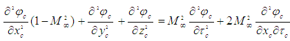
 is the local speed of sound. The wave described by (7) continues onwards to infinity since no viscosity terms are included in the formulation to dissipate the wave. Terms in (7) can be rearranged such that the second-order derivatives of the velocity potential are combined to form the following unsteady wave equation in Cartesian coordinates for compressible fluid flow [14, 15]:
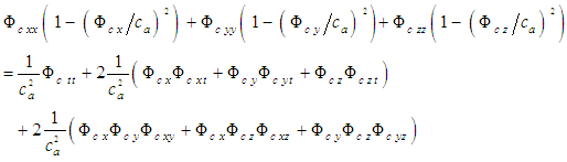 | (8) |
 and
and  in the wave equation (8) represent nonlinearities generated after differentiating squared-velocity quantities in (7). The cross-derivative terms vanish as the flow speed goes to zero but otherwise remain non-zero valued as the speed increases. Hence, any attempt to eliminate the cross derivatives by means of coordinate transformations will also make the transformed fluid a fictitious fluid. The non-dimensional variable
  is defined as the Mach number in the jth direction of flow. It is evaluated as the quotient of the fluid velocity in the jth direction and the local speed of sound
  , such that:
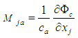 | (9) |
 | (10) |
 with one representing a free-stream or undisturbed flow speed
  (i.e., speed of the solid body) in the X-direction and that of a small perturbed velocity potential component
  . Under these conditions, the following linearized expansion using a perturbation velocity potential
  for compressible flow conditions can be used, such that:
 | (11) |
 and if flow is aligned along the X-axis. The resultant unsteady perturbation velocity potential equation reduces as follows:
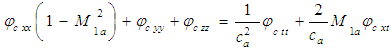 | (12) |
2.2. Steady-State Case
- The steady Prandtl-Glauert equation is obtained from the general velocity potential equation (10), such that:
 | (13) |
 is also aligned along the X-axis, such that:
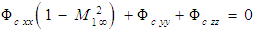 | (14) |
3. Incompressible Flow
- The more general problem of describing the convective wave equation in a compressible fluid medium will now be simplified for subsonic speeds. A brute force selection procedure will be presented to transform the coordinate system to various fictitious, incompressible flow systems. This approach will demonstrate that the resultant transformations are mathematical constructs that only depend on satisfying the desired form of the partial differential equations being transformed.Convert coordinate time intervals
 and
and  with initial times
  and
and  to distance intervals
  and
and  by introducing the following change in variables:
 | (15) |
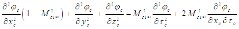 | (16) |
 in the convected wave equation (16) is defined in (9) and (11) as a function of the local perturbation velocity
  for a compressible fluid medium.The wave equation (16) for a compressible fluid with coordinate system
  will now be transformed to an equivalent incompressible flow coordinate system
 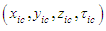 in Cartesian coordinates. Incompressible terms are indicated by using the subscript “ic”. A subsonic free-stream velocity
  and free-stream speed of sound
  in the compressible flow system will be assumed, such that:
 | (17) |
 | (18) |
 | (19) |
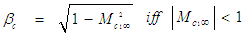
 . Note that the
  and
and  line coordinates must be defined over an infinite domain in order for these transformation methods to be valid. The coefficient
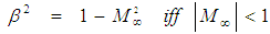
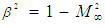
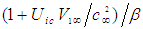
  in (17) is called the Prandtl-Glauert factor in aerodynamics and the Lorentz contraction factor in the theory of relativity [20]. It should be obvious from (19) that the new variable
  is no longer a real time variable since its value is translated by the X space coordinate term
  . This means the newly introduced
  and
and  coordinates are part of a fictitious mathematical construct that will be used to simplify the partial differential equations. Term
  is set equal to the Jacobian determinant of the
  transformation matrix given in (19):
 | (20) |
 with respect to the compressible Cartesian coordinate
  and the compressible time variable
  . Replace the coordinate derivatives in (16) using the chain rule on (19), such that:
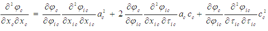 | (21) |
 | (22) |
 | (23) |
 | (24) |
 | (25) |
 | (26) |
 | (27) |
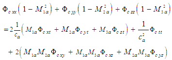
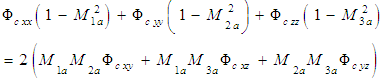
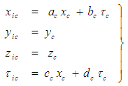
 vector is assumed to be aligned parallel with the X axis. Hence, the transformation problem reduces to finding the remaining coefficients for just the X and T components. There remain four unknown coefficients
 and four constraint equations in (24) to (27). The value of the three sign terms used in (24) to (27) are unknown but they are restricted to plus or minus one. The end product of the transformation process is a partial differential equation that represents the wave equation of the perturbation velocity potential for an incompressible fluid medium with a FTV reference frame, such that:
 | (28) |
 terms equal plus one [21].
3.1. Brute Force Algorithm
- The more general problem to be addressed here is to present a brute force algorithm that is used to perform a systematic search of coefficients for the linear homogeneous transformation with just X and T components. These coefficients will convert the convected wave equation for a compressible fluid medium with a FTV reference frame into a wave equation for an incompressible fluid medium with either a FTV or FIS reference frame. The algebraic matrix used in this search is as follows:
 | (29) |
 and
and  A search was conducted using eleven trial formulas that were substituted into the numerator coefficients
  and
and  . The eleven trial formulas are as follows:


 In addition, seven trial formulas were systematically substituted into the denominator coefficient
  The seven trial formulas are as follows:
 A systematic search using the above combination of numerator and denominator trial formulas resulted in a total of 102,487 combinations that were tested. The three sign terms used in (24) to (27) are only allowed to have values equal to plus or minus one:

 ; The search using these three sign coefficients requires an additional eight times of effort, resulting in a total of 819,896 searches. The actual search is easily performed using a numerical algorithm by setting the Mach number
  to an arbitrary subsonic value, such as 0.3, looping through all of the different formulas and signs, and saving only those trial formulas that exactly satisfy the four constraining expressions (24) to (27). Only six unique transformation sets were found during these searches. These are listed in Table 1. Term
  is the Jacobian determinant of the transformation matrix shown in the third column. Three of the transformations have a Jacobian determinant equal to plus one and three have a Jacobian determinant equal to minus one.
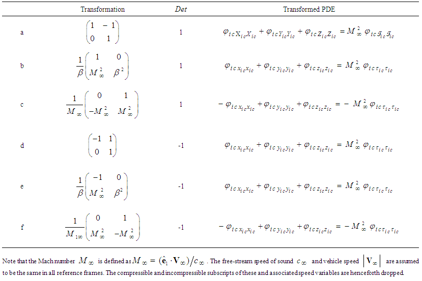 | Table 1. Summary of the six coordinate transformations that are unique and that satisfy the four constraints given in (24) to (27) |
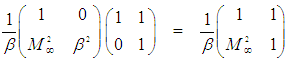 | (30) |
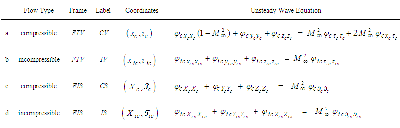 | Table 2. Partial differential equations of the unsteady, perturbation velocity potential in Cartesian coordinates |
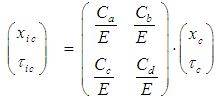
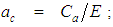
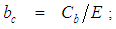
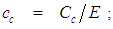
 ;
;  ;
;  ; and
; and 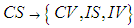 . The coefficients for these are derived in the same brute force manner previously described or by using simple substitution or inversions between matrices. These twelve transformation matrices are listed in Table 3.In a manner similar to that developed for (15), the coordinate time variables
  and
and  for a FIS reference frame are related to units of distances
  and
and  through the following change in variables:
 | (31) |
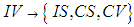
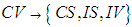
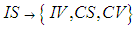
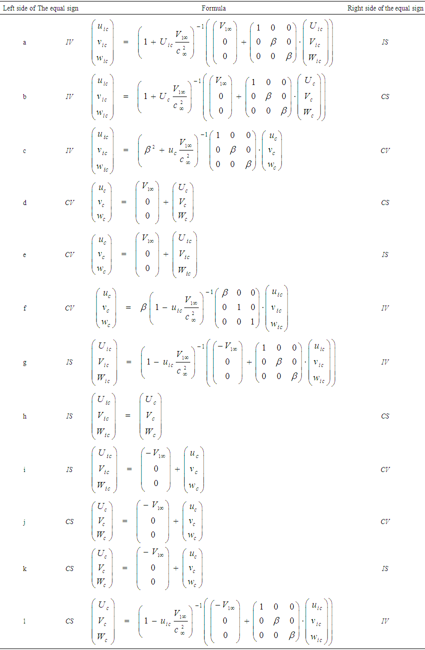
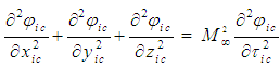
3.2. Summary of Subsonic Coordinate Transformations
- A list of the twelve transformation matrices used to convert the convected wave equation for subsonic speeds from compressible to incompressible flow conditions or the reverse process are listed in Table 3. Two letter abbreviations of the reference frame are listed in the second and fourth columns and the classical name associated with the transformation matrix is listed in the last column.It is worth repeating that only the compressible FTV (i.e., CV) wave equation with cross derivatives in Table 2 represent air as a real fluid. The other three represent the wave equations for three different fictitious fluids. The brute force algorithm used to produce Table 3 demonstrates, from a heuristic point of view, that the transformation matrices enforce a particular linkage between time and space coordinates. This linkage eliminates the generation of cross-derivative terms involving time when transforming between the compressible wave equation CV and the three fictitious wave equation CS, IV, and IS. As stated at the bottom of Table 3, the brute force algorithm assumed the speeds
 and
and  to be the same in all reference frames, i.e.,
  . However, the constraints of (24) to (27) do not require this speed constant to be the maximum allowed speed.Consider the
  transformation formulas
  for the X-coordinate and
  for the T-coordinate given on line f of Table 3. These formulas convert spatial and temporal changes measured in an incompressible flow system to changes in a compressible flow system. The Prandtl-Glauert factor
  is always less than one for subsonic speeds. It then follows that an observer working in a compressible flow system might be tempted to conclude that spatial measurement
  decreases in length and that temporal measurement
  increases in duration with an increase in the free-stream speed
  . Of course we know this is only a mathematical artefact arising from the decision that someone previously had used a theoretical model based on the assumption of incompressible flow. This is exactly the case faced by aeronautical engineers before the availability of high speed wind tunnels and fast computers to run computational fluid dynamic software before WWII. No discrepancy in measurement occurs with speed if the observer had been consistent in comparing measurements against a theoretical model based on compressible flow. However, the situation is much more difficult and paradoxical to resolve if the observer were to deny the very existence of a compressible flow system. Space and time would then be concluded to be warped or bent with speed.
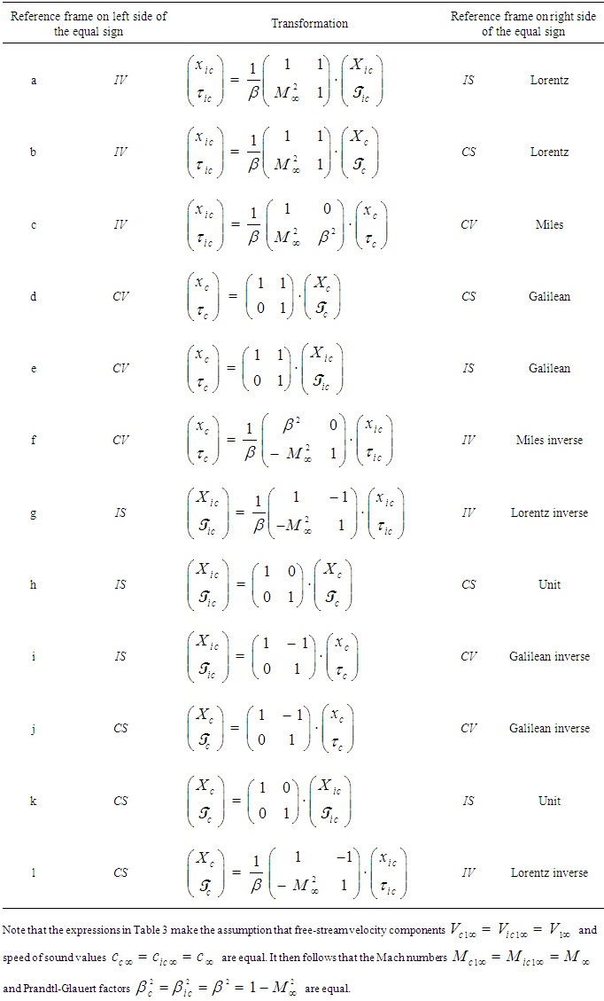 | Table 3. Summary of coordinate transformations for subsonic flow conditions |
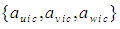
3.3. Velocity Transforms between Reference Frames
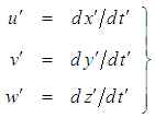
- This section will describe how the perturbed velocity components developed in one reference frame can be related to those in another reference frame using the various coordinate transformations introduced in the previous section. The basic approach of [20] will be followed.Let there be two different reference frames, called the
 and
and  systems. Assume the
  system moves relative to the
  system with velocity
  in a direction that is parallel to the X-axis of both systems. Define the X-axis velocity component
  as the particle velocity for the
  system and the X-axis velocity component
  of the same particle in the
  system, such that in general:
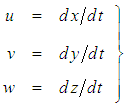 | (32) |
 | (33) |
3.4. Transforming Velocities from FIS to FTV Reference Frames
- The transformation between FIS and FTV reference frames is represented by the matrix on line a of Table 3 for incompressible flow systems, such that upon taking incremental differences in the coordinates:
 | (34) |
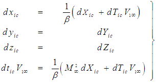 | (35) |
 associated with the FTV reference frame and
  associated with the FIS reference frame are related to incremental changes in coordinate time variables
  and
and  by the relationships (15) and (31), such that:
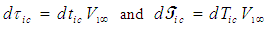 | (36) |
 from the fourth line in (35), such that:
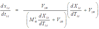 | (37) |
 | (38) |
 | (39) |
 of the FTV reference frame for an incompressible flow system using expressions from (5) and (37):
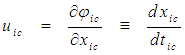 | (40) |
 | (41) |
 | (42) |
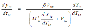
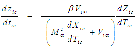
 of the FIS reference frame for an incompressible flow system:
 | (43) |
 | (44) |
 | (45) |
 with
with  , and rearrange the resultant terms, such that for incompressible flow systems:
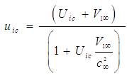 | (46) |
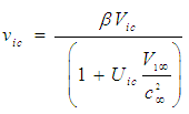 | (47) |
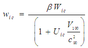 | (48) |
 &
&  . The expressions in (46) through (48) are collectively called the velocity-addition formulas [20] or the composition law for velocities. They are mathematical manifestations of the Lorentz transformation used in (30) to transform the FIS reference frame to a FTV reference frame in incompressible flow systems. It is easy to show with numerical simulation that the magnitude of the perturbed velocity set
  in formulas (46) to (48) will always vary between 0 and the fluid’s characteristic speed
  when the magnitude of the FIS perturbation velocity set
 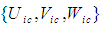 varies between 0 and
  ; and when the magnitude of the free-stream velocity
  is restricted to vary between 0 and
  .Consider for a moment the simple coordinate modification for the FTV and FIS velocity representations in the X-Y plane of the incompressible flow system:
  ,
,  ,
,  , and
, and  . Substitute these trigonometric relationships into the Y-axis component of (47):
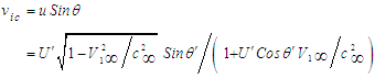 | (49) |
 is much less than one such that:
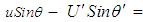
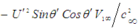 . Further assume the special case where the velocity components
  and
and  are equal to speed
 Substitute in the sine subtracting function
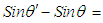
 , such that:
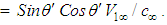 Define
 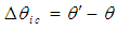 as the difference between the velocity coordinate angles
  and
and  in the X-Y plane of the incompressible flow system. The
 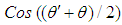 and
and  terms cancel each other when
  goes to zero, such that:
 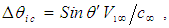 where
where 
 and
and  This final expression for
  is called the aberration of light formula in relativistic physics [20] when
  is interpreted as the speed of light in vacuum.Now consider the relationship between the speed of the FTV perturbation velocity set
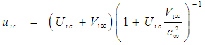
  and the speed of the FIS perturbation set
  Define the FTV speed
  and FIS speed
  for incompressible flow as follows:
 | (50) |
 | (51) |
 in (50), such that:
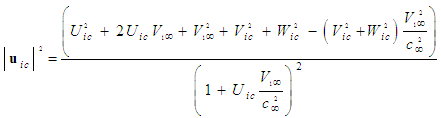 | (52) |
 from (52) into the formula
  and take the square root of the resultant expression, such that for incompressible flow:
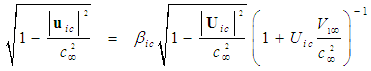 | (53) |
 can be derived with the help of (51) as follows:
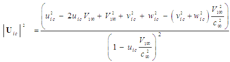 | (54) |
 is given by:
 | (55) |
 and multiply the resultant expressions together, such that:
 | (56) |
3.5. Summary of Subsonic Velocity Transforms
- This section summarizes in Table 4 all twelve of the velocity relationships developed from the twelve coordinate transformations listed in Table 3 for subsonic speeds.
 | Table 4. Summary of subsonic velocity transformations when using FTV versus FIS reference frames and compressible versus incompressible flow systems |
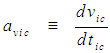
3.6. Transforming Velocities from FIS to FTV Reference Frames
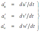
- This section describes how the perturbed acceleration components developed in one reference frame can be related to those in another using the various transformations introduced in the previous sections. Let there be two different reference frames, called the
 and
and  systems. Assume the
  system moves relative to the
  system with constant velocity
  in a direction that is parallel to the X-axis of both systems. Define the X-axis acceleration component
  as the particle acceleration for the
  system and the X-axis acceleration component
  of the same particle in the
  system, such that in general:
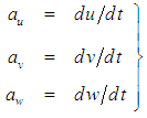 | (57) |
 | (58) |
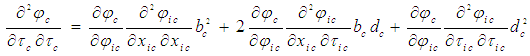
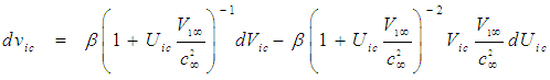
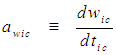
3.6.1. Transforming Accelerations from FIS to FTV Reference Frames
- Make an incremental change in the velocity terms
 and
and  in the matrix of line a in Table 4, keeping the free-stream velocity
  and speed
  constant, such that:
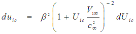 | (59) |
 | (60) |
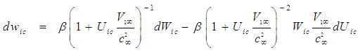 | (61) |
 from the fourth line in (35) and on the right side of the equal sign by
 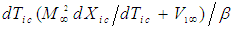 , such that for incompressible flow:
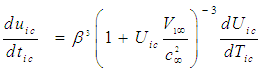 | (62) |
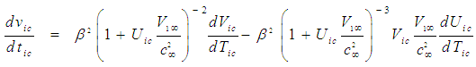 | (63) |
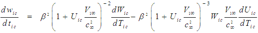 | (64) |
 of the FTV reference frame for an incompressible flow system, such that:
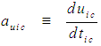 | (65) |
 | (66) |
 | (67) |
 of the FIS reference frame for an incompressible flow system, such that:
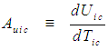 | (68) |
 | (69) |
 | (70) |
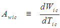
 | Table 5. Summary of subsonic acceleration transformations as a function of using fixed-to-vehicle versus fixed-in-space reference frames and compressible versus incompressible flow systems |
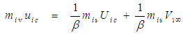
3.7. Transforms of Momentum and Fluid Mass between Reference Frames
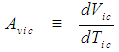
- This section describes how the momentum and fluid mass components developed in one reference frame can be related to those in another using the various transformations previously described. Linear momentum vector
 of an infinitesimal volume of fluid is defined as the mass
  of the infinitesimal fluid volume times the fluid perturbation velocity vector
  , such that
  .
.3.7.1. Vectors Defined for Incompressible Flow Systems
- Define vector set
 to represent the momentum components when evaluated in a FIS reference frame for incompressible flow conditions, such that
  . Term
  represents the fluid mass of an infinitesimal volume of fluid when evaluated with a FIS reference frame for incompressible flow conditions. Define vector set
 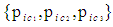 to represent the momentum components evaluated with a FTV reference frame for incompressible flow conditions, such that
 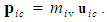 Term
Term  represents the fluid mass of an infinitesimal volume of fluid when evaluated with a FTV reference frame for incompressible flow conditions.
3.7.2. Vectors Defined for Compressible Flow Systems
- In a similar manner, define vector set
 to represent the momentum components when evaluated with a FIS reference frame for compressible flow conditions, such that
  . Term
  represents the fluid mass of an infinitesimal volume of fluid when evaluated with a FIS reference frame for compressible flow conditions. Let vector set
  represent the momentum components evaluated with a FTV reference frame for compressible flow conditions, such that
  . Term
  represents the fluid mass of an infinitesimal volume of fluid when evaluated with a FTV reference frame for compressible flow conditions.
3.7.3. Coordinate System and Reference Frame Transforms
- Assume the momentum terms for incompressible flow in the FIS reference frame are related by a transformation to the incompressible flow system in a FTV reference frame in the following manner when the free-stream flow (with speed
 ) is parallel to the X-axis:
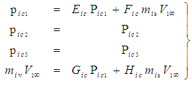 | (71) |
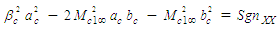
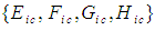 in (71) are unknown constants. The Jacobian determinant of the matrix in (71) must equal a value of plus one, such that:
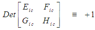 | (72) |
 | (73) |
 | (74) |
 and rearrange terms to solve for the fluid mass
  in an incompressible flow system and a FTV reference frame, such that:
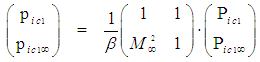
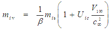 | (75) |
 from (53) into (75) and rearrange terms, such that:
 | (76) |
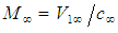
 is called the rest mass. It represents the fluid’s mass when the fluid at a particular point is brought to zero-speed conditions in the incompressible flow system. Hence, a relationship can be developed for the fluid mass in either the FTV or FIS reference frames of incompressible flow by rearranging (76), such that:
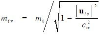 | (77) |
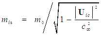 | (78) |
 or FIS velocity
  perturbation velocity vectors approach the characteristic speed
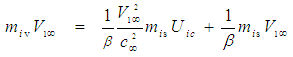
  . Clearly predicting an infinite increase in mass as the free-stream speed increases is not physically meaningful since the linearized expressions used in the derivation for potential flow are no longer valid. Modern day jet airplanes are quite capable of flying at both transonic and supersonic speeds without gaining an infinite mass.The momentum vector
  in the FTV reference frame for an incompressible flow system can now be expressed in terms of the rest mass
  by substituting (77) for mass
  back into the definition (69), such that:
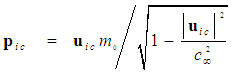 | (79) |
 in the FIS reference frame for an incompressible flow system can now be expressed in terms of the rest mass
  by substituting (78) for mass
  back into the definition (70), such that:
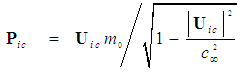 | (80) |
3.7.4. Verifying Fluid Mass Formulation
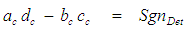
- The approach presented in the previous section that derived the fluid mass for an incompressible flow system will now be verified. Write out the first line of either (71) or (73) for momentum, such that:
 | (81) |
 in (81) with (77) and mass term
  with (78), such that:
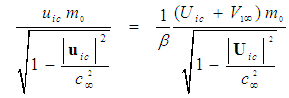 | (82) |
 | (83) |
 velocity component for an incompressible flow system with a FTV coordinate frame matches exactly that given by the
  transformation matrix listed on line a of Table 4.
3.7.5. Summary of Subsonic Fluid Mass Transformations
- A summary for the twelve reference frame formulas used for fluid mass transformations is given in Table 6.
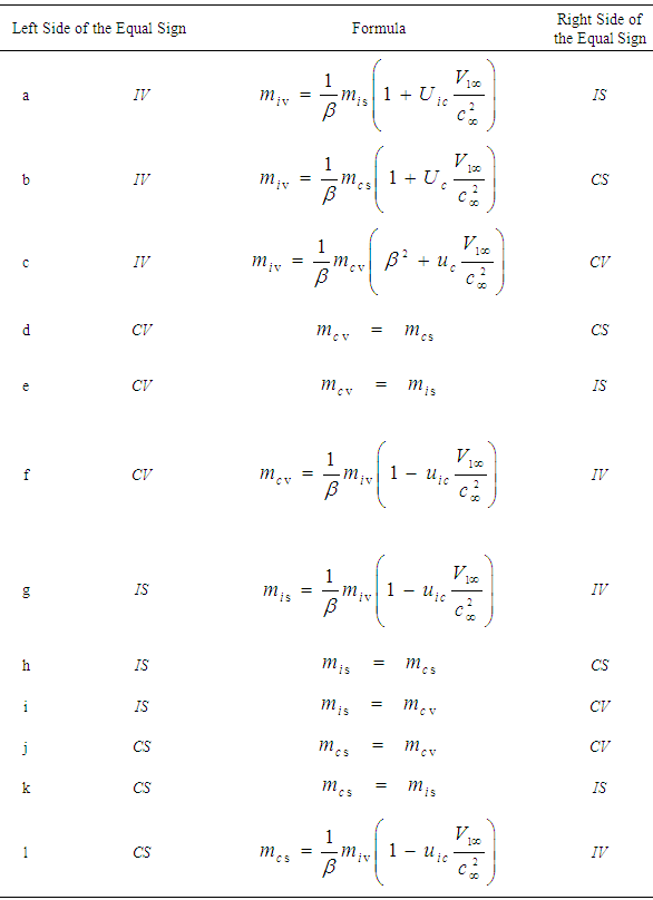 | Table 6. Summary of subsonic fluid mass transformations as a function of using FTV versus FIS reference frames and compressible versus incompressible flow systems |
4. Summary
- The paper starts by reviewing the wide spread use of Prandtl-Glauert correction factors by aeronautical engineers before World War II. Correction factors were needed to account for the effects of compressibility as a function of subsonic air speeds when using theoretical formulas based on an incompressible flow theory. This approach fell out of favor with the introduction of jet engines that could propel aircraft from subsonic to supersonic speeds. Engineers now use computational fluid dynamic algorithms to solve the complete Navier-Stokes equations that explicitly include all of the compressibility effects.A more detailed examination of the mathematics behind the origin of the correction factors reveals a profound analogy to the equations of special relativity. To see this connection, a derivation of the classical three dimensional, convected wave equation is given in Cartesian coordinates representing the disturbance produced by the subsonic movement of a slender, solid object through still air with velocity
 . The velocity potential of the disturbed air is solved under the assumptions of compressible flow conditions and a fixed-to-vehicle (FTV) coordinate reference frame, abbreviated as reference frame CV. Atmospheric air is assumed to have the properties of irrotational, inviscid, barotropic, isentropic flow conditions; all external forces such as gravity are negligible; and the characteristic speed
  of free-stream air is constant. In order to simplify the expressions, the vehicle velocity
  is aligned along the X-axis of the coordinate system. Four partial differential equations for the transient wave equation of perturbed velocity potential are presented to represent alternative reference frames labeled as CV (compressible-FTV), CS (compressible-FIS), IV (incompressible-FTV), and IS (incompressible-FIS). Only the X space and T time coordinate components of the partial differential equations vary between the different reference frames. A brute force algorithm is described that searches for the coefficients of the 2x2 linear transformation matrices with a unit Jacobian determinant to convert the partial differential equation in reference frame CV to those of frames CS, IV, and IS. There are a total of twelve matrices needed to describe both forward and reverse transformations between the four reference frames. After trying approximately one million combination of terms, only the coefficients for three unique transformation matrices are found: the unit, inverse Galilean, and Miles matrices. The Lorentz matrix is obtained by multiplying the Galilean and Miles matrices together. Incremental differences in all of the space and time terms in the coordinate transformation matrices are taken. Expressions for the twelve 3x3 velocity transformation matrices are found by dividing the dX coordinate equation in each matrix by the corresponding dT equation. Similar steps are used to derive expressions for twelve 3x3 acceleration transformation matrices, and finally twelve 1x1 fluid mass transformation matrices.Every transformation matrix shown in Tables 4 to 6 has an inverse form for itself. If
  represents the ith matrix in one of these three tables, then the dot product of the matrices
 and
and  equals the identity matrix. In addition, linking the dot products of all twelve matrices from a given table into a certain order, such as the sequence
 will produce a circular chain returning to the same coordinates that it started with.
5. Discussion
- It is worth the effort to compare the form of the convected wave equation describing compressible flow in (84) against the form of the wave equation for incompressible flow in (85) (i.e., the analogous equation used in electromagnetic theory):
 | (84) |
 | (85) |
 and XT cross-derivative in (84) resemble a type of rococo styled mathematics. Surely (85) is the true form of the equation representing the simplest expression for electromagnetic wave propagation. Why would it ever need to be more complicated? However, only (84) accounts for the effect of fluid compressibility in an absolute coordinate system of space and time. Removing the extra coefficient and cross-derivative by means of a coordinate transformation renders (85) an expression for a fictitious fluid and for space and time coordinates that change in magnitude as a function of speed.It took many years for the majority of the public and scientific community to accept both heavier-than-air flight and faster-than-sound flight before WWII. Acceptance was stymied by arguments put forward to society through the popular press that were often based on political or religious ideology and parsimonious logic (i.e., if God intended man to fly he would have given us wings).As another example, the use and interpretation of coordinate transformations can be confounded by using distance and time measuring devices that are also affected by the compressibility of the media itself. If one used an acoustic timing device in an inflight vehicle connected to outside conditions, its time delay measurements would also be affected by changes in air compressibility as speed varied. It then follows that if one rejects the hypotheses of speed affecting air compressibility, then discrepancies in the time delay measurements from the acoustic device would falsely be interpreted as space and time coordinates being bent.The derivations given herein demonstrate that the Lorentz factor is not special in the normal sense of the word. Rather, it is a compressibility correction factor arising from the consequence of ignoring compressibility in the formulation of the convected wave equation. When compressibility is ignored, then correction factors are needed to compensate for the mathematical artefacts arising from spatial contraction and temporal dilation. In addition, velocity, acceleration, and mass vary with speed and no longer obey simple addition rules. The story of subsonic compressible aerodynamics is presented here because some of the same theoretical and mathematical developments occurring in manned flight were occurring almost simultaneously in the field of physics. The difference between the evolution of theory in aerodynamics and physics is that the majority of aerodynamists have accepted the concept of air compressibility but the majority of physicists have rejected the concept of vacuo compressibility.
6. Conclusions
- Twelve coordinate transformations, plus formulas for subsonic velocity, acceleration, and mass are derived entirely from a brute force iteration routine using the mathematical characteristics of the partial differential equations from classical fluid dynamics for compressible flow and its transformation to incompressible flow. The mathematical derivation and interpretation for the twelve sets of transforms are apparently new. In addition, it was shown that there was no need to introduce additional assumptions concerning the positioning and timing between clocks, chord lengths, and speeding planes.Examination of the formulas for coordinate transformation, velocity addition, and mass equations for subsonic conditions shows the equations are mathematically identical to those used in special relative to describe the motion of an electromagnetic wave or a particle, with the speed of light in vacuum used in place of the speed of sound for air. The convected wave equation for compressible flow and the special relativity wave equation only match exactly if the special relativity equations are assumed to be based on vacuum conditions, where the vacuum is represented by an incompressible flow system with a fixed-in-space reference frame (IS).The proper starting form for using the convected wave equation is the form which includes cross derivatives in time and space. Any mathematical transform that removes these cross derivatives will convert the resultant equation into a non-physical form that represents a fictitious fluid.