Witold Nawrot
Correspondence to: Witold Nawrot, .
| Email: |  |
Copyright © 2017 Scientific & Academic Publishing. All Rights Reserved.
This work is licensed under the Creative Commons Attribution International License (CC BY).
http://creativecommons.org/licenses/by/4.0/

Abstract
A new, alternative idea of the reality is presented. Instead of four-dimensional space-time with the signature defined with the metric tensor and dimensions deformed as a function of body’s motion, a four-dimensional absolute Euclidean space is proposed whose dimensions do not have a predetermined meaning of time or space. The dimensions of time and space are not the dimensions creating the reality any more, but they are only certain directions in Euclidean four-dimensional space. And these directions depend on the pair of observer – observed body. While observing bodies moving with various velocities we interpret various directions in the Euclidean reality as the space-time dimensions and that’s, in general, the difference of directions interpreted by us as the space-time dimensions and not the deformation of dimensions, becomes responsible for relativistic phenomena. The new approach significantly simplifies the description of reality – through the description in Euclidean space, it eliminates singularities and additionally answers many questions that the Theory of Relativity was not able to answer to for almost 100 years.
Keywords:
Euclidean relativity, Recession of galaxies, Dark energy, Time dilation, Lorentz transformation, Mach principle, Wave function
Cite this paper: Witold Nawrot, Alternative Idea of Relativity, International Journal of Theoretical and Mathematical Physics, Vol. 7 No. 5, 2017, pp. 95-112. doi: 10.5923/j.ijtmp.20170705.01.
1. Introduction
I have been working for years on creating a model of reality alternative to the model introduced by the Theory of Relativity. The motivation for undertaking the construction of a new model from the ground up instead of developing the existing Theory of Relativity was the unnecessary complexity of the model, excessive number of assumptions and postulates, and accepting certain phenomena as the basis for further consideration instead of searching for the sources of these phenomena, and the fact that the current model leaves many questions and doubts which, despite the fact that TR was created more than 100 years ago, have still not been answered.I wanted to begin the list of doubts and objections regarding the Theory of Relativity from the well-known problems, widely discussed over the years: The first problem is that the Lorentz transformation predicts time dilation and the length contraction. Even though we can see the proof of the time dilation every day while driving and using GPS navigation, length contraction of objects in motion has not been confirmed so far.The next problem is the recession of galaxies - RT cannot explain this phenomenon. One of the attempts at explaining the phenomenon of recession of galaxies assumes the existence of the so-called dark energy, which has not been detected. It remains to be clarified whether the observed increase in the speed of galaxies as a function of distance is a result of actual acceleration of galaxies or whether it's the result of some unknown phenomena related to the way of observing reality. The Mach principle and the fact that it is impossible to explain it within TR is also one of the problems.And the next issue I would like to mention is the lack of connection between Quantum Mechanics and the Theory of Relativity. If the TR is a theory that properly describes the reality that surrounds us, then at some point the effects described by the QM should appear. But so far, those are two separate models describing different types of phenomena.There is also a problem with the existence of singularities in the TR. The existence of infinite values in the true reality does not seem to be possible. Perhaps the singularities are not the property of the reality but they result only from the properties of the current model, i.e. they are the properties of the accepted description. Perhaps, accepting another model would allow to avoid singularities in the description.To the above well-known problems I would like to add a few of my personal remarks and doubts:I would like to start from the covariant notation itself. The introduction of time as a fourth dimension to the description of the reality was based on the introduction of a metric tensor with the signature 1-1-1-1, whose form was chosen to assure compatibility with the observations. However, there is no deeper justification for this and not another form of metric tensor. The use of metric tensor does not explain the source of any phenomenon. It only says: if-then, therefore it describes the problems and does not explain them. To justify my view of this problem I can give the following example: if I wanted to describe how the lights in my room work, I could define the tensor, analogous to the metric tensor, with the signature of zeros and ones, for instance 111101101, where zero corresponds to a broken bulb, and one to a good one. This signature, is accepted because it is consistent with the observation of the behavior of the lights (we do not need to know how the bulb works or what the construction of the bulbs is). Multiplying this tensor by a zero-one vector of the state of switches, we get a description of the operation of the lights. Such a method allows us to describe the operation of the lights. But does it allow us to understand the essence of electricity? Of course not, there is no Ohm’s law, electric potentials, motion of electrons, electrical charges, quantum emission, etc. Meanwhile, this kind of description is the basis we use for building the relativistic equations. By applying the tensor notation we can describe practically all physical phenomena - analogous to the description of electricity described above - but it is always a description only. Of course it will allow us in many cases, to draw conclusions about behavior of the phenomena under new conditions; however, it is still just a description and not an explanation of the essence of the phenomenon.Another problem is the premature - in my opinion - acceptance of the postulate of constancy of the speed of light. Accepting this postulate allowed, on the one hand, to quite quickly develop the Theory of Relativity to its present form and to achieve many spectacular successes with the TR at the beginning of the last century; however, it also blocked research on the physics that is responsible for the phenomenon of constancy of the speed light. Of course, such research would have delayed the development of the RT at an early stage, but resolving the problem of constancy of the speed of light instead of adopting it as a postulate would probably allow knowledge to progress further than it has in this past century. If the velocity of light behaves strangely from our point of view – i.e. is constant regardless of the velocity of the observer – then, when solving this problem, we do not need to match the model to the observed phenomena at the cost of complexity and accepting many unexplained phenomena as basic assumptions and postulates. Perhaps the use of the notion of velocity should be limited only to non-relativistic mechanics - hence the unusual behavior of velocity of light for higher velocities of observers. Maybe instead of adjusting and complicating the model to fit the familiar notions of velocity to the relativistic phenomena - to which this notion may not apply - we should think about describing the relativistic motion with another, yet unknown, variable? Finally, about 500 years ago, attempts were made to adapt the model describing the motion of the planets to their motions observed on the firmament, which led to the unnecessarily complicated model describing the motion of the heavenly bodies. It was enough to move the reference system from Earth to the Sun for everything to become easy to explain. In case of velocity we may be dealing with a similar mechanism.Another problem is the time dilation as a function of the motion of bodies. In the TR it is accepted that the time in a frame in motion slows according to the following formula:  | (1) |
where  – time in the frame in motion,
  - time in the frame of an observer.Multiple experiments confirmed this relationship. However, this experimental evidence has one fundamental flaw, which I already described in my previous papers [1, 2] namely in the experiment of Hafele and Keating from 1971, and in case of the motions of GPS satellites, this formula is true only for curved routes. Therefore, these experiments are an evidence for the General Theory of Relativity and cannot be treated as a proof for the time dilation for rectilinear and constant motion, i.e. for the STR – as it is currently accepted. Moreover, the mistake made by Hafele and Keating while deriving formula (1) with the help of the STR is also repeated in case of other experiments which prove the correctness of the time dilation as a function of velocity. Therefore, currently we are not able to unequivocally state if the formula (1) proves that the uniform, rectilinear motion is responsible for time dilation, because during the experiment one of the participants must change its velocity to register the actual time difference, and it is very likely that this velocity change is responsible for the mechanism of actual dilation of time.As one can see, though the TR is describing many phenomena correctly and has been successful in many areas, there are some important issues that do not seem to be solved within the TR.
2. The Basis of the New Approach to Problems of Space-Time
It turns out that it is possible to create a model of reality that, apart from explaining the problems described by the "classical" Theory of Relativity, also allows to answer all the questions and doubts mentioned above. While there are still problems that have not been completely resolved, it can be said that the milestones have been developed for the new model of reality which allows to simplify the description of phenomena and expands the description potential, within one model, for a wider range of phenomena than before. Arguments for seriously considering the approach proposed below include greatly simplified description of many phenomena, the possibility of describing and solving, within one model, many problems and phenomena, such as the recession of galaxies, time dilation, Mach principle, wave properties of particles, etc., which up till now required different models, a significantly wider scope of described phenomena in relation to the capacity of the Theory of Relativity, and the fact that the new model in its current state can be experimentally verified.The essence of the idea presented here relies on the assumption that the "true" reality is built of different dimensions than the observed dimensions of time and space, namely:1. The “true” reality is a four-dimensional, absolute Euclidean space, its dimensions denote certain distances, which do not have the meaning of time or space distances assigned in advance. The dimensions creating the four-dimensional absolute Euclidean space will be marked with letters abcd to distinguish them from dimensions of time and space – xyzt, perceived by us. The four-dimensional, absolute Euclidean space described with the letters abcd, together with bodies existing in it, in further parts of this paper will be named FER – Four-dimensional Euclidean Reality. The notion “space-time”, in this paper, will denote the “traditional” four-dimensional Minkowski space-time.2. The space-time dimensions xyzt (because of the lack of covariant notation, for the purpose of this article I will not be marking space-time dimensions as “xi”, etc.), in this model, are not the dimensions creating the reality any more. The dimensions xyzt observed by us are nothing more than certain directions in the “true” Euclidean reality (FER); these directions are not stable but depend on the observer and the currently observed bodies. The rules for defining the space-time dimensions in the FER will be described in the following points. 3. In the four-dimensional absolute reality (FER), there are bodies. These bodies are “moving” along trajectories in the FER (the notion of “trajectory” in the FER replaces the notion of “world line”, which is proper for the space-time). The term "move" means that in case of rectilinear trajectories, the length of the trajectory traveled by the body is the measure of proper time of this body. Trajectory for a specified body has a direction and order and is interpreted by the body as its time dimension. All trajectories are allowed and equivalent. 4. As the space-dimensions we interpret three directions in FER orthogonal to each other, perpendicular to the trajectory of the currently observed body. It means that the observer, while observing different bodies, interprets different directions in the FER as its space-dimensions. Thus, in FER, in relativistic cases, for observation of each specific body, a different set of directions interpreted as the space coordinates is defined, and the direction interpreted as the time dimension (the trajectory of an observer) is not, in general, perpendicular (in FER) to the directions interpreted as the space-dimensions (see for instance Fig. 1). This is an illustration of the fact that the dimensions themselves cannot be observed, and we learn about the existence of space and the number of its dimensions through observation of the surrounding bodies.5. The idea of absolute space needs to be complemented with the concept of an absolute time. The absolute time is not the fifth dimension. It is a parameter and corresponds to the distance between points in the FER. In the case of rectilinear trajectories, the absolute time is equal to the time that passed in the coordinate system of the body moving along that trajectory.I will show how the new model works using specific problems as examples.
3. Absolute and Relative Motion. Speed, Mach Principle, Singularities
From the assumptions above it follows that bodies exist in the FER and move along trajectories – for the time being, rectilinear. According to the assumptions, the “motion” means travelling along the trajectory, and the length of the trajectory traveled by a body is equal to the time measured by the clock of that body. Therefore, in case of rectilinear trajectories, each body moves relative to the absolute space at an absolute velocity equal to 1. Since the measure of time of a body is the length of the trajectory traveled by this body, then the motion of the body relative to the absolute space is interpreted by the body as the time flow, and the trajectory in FER is the time axis of the body’s coordinate system.Now, if two bodies move along trajectories inclined to each other at an angle then the observer interprets directions perpendicular to the trajectory of the observed body as its space-dimensions. This situation is presented in Figure 1.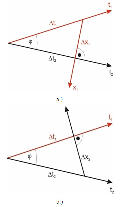 | Figure 1. Mutual observation of bodies. Two bodies move along their trajectories which are the time axes of their local coordinate systems. The FER directions perpendicular to the trajectory (the time axis) of the observed body are interpreted by the observer as its space-dimensions. In Fig. a, the body 1 is the observer (coordinate system x1t1); in Fig. b, the body 2 is the observer (coordinate system x2t2). In FER, for relativistic cases the time axis of the observer is not perpendicular to its space dimensions |
Due to the proposed way of observing bodies along the directions perpendicular to the trajectory of the observed body, although the space is absolute and the motion of the bodies relative to space is absolute, the mutual motion of the bodies is relative and is described not by the motion relative to space but by the angle between the trajectories of the bodies. Looking at Fig.1, we can see that the relative velocity of bodies is described with formula (2)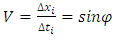 | (2) |
where i=1,2.From this formula and the mechanism of observation shown above, a number of instant conclusions can be drawn:1. The relative motion of bodies measured by the relative inclination of the trajectories of the bodies, and the absolute motion relative to the space, i.e. the motion of the bodies along their trajectories, are distinct phenomena that are not mutually exclusive each other.2. Since all the trajectories are equivalent, the physical phenomena cannot depend on the angle of the trajectory in the FER, i.e. on the relative speed, and this automatically fulfills the first postulate of the TR.3. The absence of a distinguished direction in the FER indicates that there is no absolute angle of inclination of the trajectory, i.e. the rectilinear motion of the bodies in the sense of formula (2) is relative -the angle of inclination of the trajectory can be determined only with respect to the trajectory of another body. In other words, the velocity measured according to the formula (2) can be determined only in relation to another object. However, in case of non-inertial motions – along a curved trajectory - the radius of curvature of the trajectory does not depend on the choice of any observer’s reference frame in the FER, because the radius of curvature of trajectory is determined in relation to the previous parts of the same trajectory, i.e. a specified trajectory, and it can be described with the absolute Euclidean coordinate system abcd.For instance, in a two-dimensional plane, the curved trajectory can be described with the formula which depends only on the absolute coordinates  (where a and b are the absolute coordinates). Then the radius of curvature will be equal to:
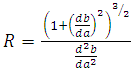 | (3) |
The radius of curvature of the trajectory does not depend on the choice of the observer. Therefore, it is an absolute value. Since the inertial forces depend on the curvature of the trajectory, the existence of the inertial forces is a consequence of existence of absolute reality or, in other words the existence of the whole Universe. It is an idea similar to the Mach principle; however, it is connected with the existence and structure of absolute space and not with the mass distribution in the Universe. So, according to the presented model, the Mach principle in general is correct but there are some important differences. The chapter “Example: The quantized time dilation in case of twin paradox” suggests some idea about how the interaction of bodies with the rest of the Universe causes inertial forces. Due to the absolute property of curvature of trajectory of bodies, which unequivocally determines the non-inertial observer, the relativity of motion in the sense known from the Theory of Relativity can be applied only for rectilinear trajectories, i.e. for inertial motions. 4. The velocity defined by the formula (2) is limited to a value of 1 – which, as it is easy to guess, is the speed of light; it will be described in detail in the following chapters (the speed of light is equal to one because all dimensions are in the same scale). This limitation means that the velocity can only be defined for trajectories inclined to the observer’s trajectory at an angle less than 90°. This is not a limitation regarding trajectory, because all trajectories are allowed. This is a limitation concerning only the observation performed in the xyzt coordinate system (space-time): it means that we are unable to observe bodies moving along trajectories inclined to the trajectory of the observer at an angle 90° and greater. It is still possible to accelerate the body to the trajectory inclined to an observer's trajectory at an angle greater than 90°; however, observation of transition to such trajectory will last until infinity and the time in the accelerated body’s frame will be observed as if it was decreasing to zero (the problem of time dilation will also be discussed later). It will result in singularities specific to the speed of light. To summarize this point: To describe the motion of bodies, a trajectory is a more general notion than velocity and allows to describe a broader class of motions, while singularities do not occur in the FER. The singularities appear only during transformation to description using space-time xyzt coordinates, when the trajectory of the observed body becomes perpendicular to the trajectory of the observer. Singularities are the result of a specific process of performing observations of bodies – with the use of directions (interpreted as the space coordinates) perpendicular to the trajectory of the observed body – and are only the property of the Minkowski model of space-time.
4. The Speed of Light
The limit of velocity for bodies defined by formula (2) is equal to 1. According to the model presented here, the velocity of propagation of the interactions is also equal to 1, but it results from a completely different mechanism.In my earlier papers [3] I suggested that quanta are sent by the observed body perpendicularly to its trajectory, i.e. along the spatial axis of the observer, and the quanta propagate along this axis at a constant velocity equal to 1 relative to that axis. This axis is then "carried” along the observer’s trajectory. Thus, the resulting trajectory of quantum in FER depends on the trajectory of the body sending the signal and the trajectory of the body receiving that signal. This mechanism is shown in Fig. 2. It shows why the speed of light does not depend on the angle between the trajectories of the bodies, i.e. the velocity. The dependence of the resultant trajectory of quantum in the FER from the trajectory of the body receiving the quantum suggests, however, the existence of instantaneous communication between quantum-communicating bodies.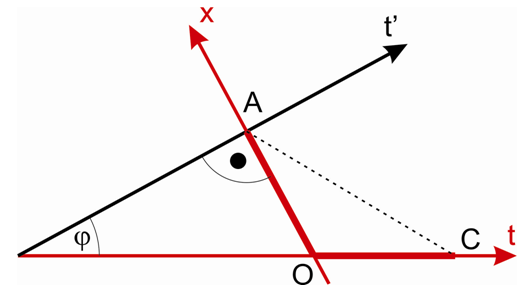 | Figure 2. Propagation of light in FER. The quantum is sent in point A by a body moving along trajectory t’. The quantum is propagating along the x-axis of the observer – the AO segment. This axis is “carried” along the trajectory of the observer – t. The resultant trajectory of the quantum is represented by the AC segment. The segments AO and OC are equal |
It has recently been found that it is possible to justify such quantum behavior in a much simpler way and without making assumptions about instant communication.It is enough to assume that bodies send and receive signals along directions perpendicular to their trajectories in FER. A body moving along its trajectory in the FER sends a signal. The signal propagates along the space direction perpendicular to the trajectory of the body at the speed of 1. Since the body keeps moving along its trajectory, the signal propagates also along the trajectory of the body at the speed of 1. Thus, the signal propagates at an angle 45° to the trajectory of the body sending the signal at an absolute velocity equal to  A similar mechanism takes place for the body receiving the signal. The described situation for pair of observers – sender and recipient of the signal - is shown in Fig. 3. At the beginning, both bodies (sender and recipient) are in the common point S.Now, if the observer in the coordinate system x1t1 positioned on the trajectory at point A (Fig. 3) sends a signal, the signal propagates along the segment AD and then along the segment DC in the FER. Namely, the signal travels the distance d along the trajectory t1 and the distance d along the direction x1 perpendicular to t1. Halfway, the spatial directions of both bodies, the one sending and the one receiving the signal, have a common point - point D in Figure 3. From this point on, the signal can propagate along the direction perpendicular to the trajectory of the body receiving the signal and, again, the signal is traveling the distance d along the direction x2 and the distance d along the trajectory t2 and finally reaches point C. Thus, in absolute space, the signal traveled distance 2d along the trajectories of the bodies, and the distance 2d along the directions perpendicular to those trajectories, interpreted as the space-dimensions of the local coordinates systems of both bodies - sender and recipient of the signal.Therefore, the above can be expressed with the formula:
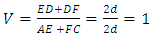 | (4) |
Where V – velocity of signal registered by observers, described in the system of absolute coordinates, and the segments AE and BF are equal to each other.Thus, considering the motion of the signals in the absolute space, we have a constant speed of propagation of the signals, regardless of the angle between the trajectories of the bodies. At the same time, the signal sent at point A on trajectory t1 reaches the trajectory t2 at point C, identical to that in Figure 2. The segments AO and OC on both figures are identical.The flaw of this model is that it works correctly only when the line defined by the SD segment is the bisector of the angle between the trajectories, which means that in practice both bodies should meet at the same point in the FER (here – point S). This problem has not yet been completely solved, but this example shows that under the above conditions, assuming propagation of signals only along directions perpendicular to the trajectories of the bodies, the constancy of the speed of light can be explained independently of the relative speed (an angle between trajectories) of the source and the receiver. At the same time, it is easy to see that for trajectories inclined to each other at an angle ≥ 90°, the signal never reaches the recipient, i.e. we are not able to observe, with the help of quantum, objects moving along such trajectories; in Fig. 3 for the angle between trajectories t1 and t2 equal to 90°, the quanta’s trajectory (AD) will be parallel to the bisector of the angle between the trajectories (SD), so the transition of the signal to the coordinate system x2t2 will not be possible. However, even though we are unable to observe these bodies, we can interact with them - for example, through collisions. There is another problem: the non-visible part of the Universe (particles/objects moving along trajectories inclined to the trajectory to observer at an angle 90°-180°) should carry additional mass similar to the mass of the observed part of the Universe. Will this additional mass affect processes in the visible part of our Universe, and if so, how? At this moment, it is difficult to answer these questions clearly, but, as we see, the new model allows for many more tools for describing and interpreting various phenomena than were previously available.We have considered propagation of signals in the absolute space FER. The velocities at which the observers move along their trajectories are equal to 1, the velocities of the signals are equal to  and the trajectories of the signals are inclined to the trajectories of the bodies sending/receiving signals at an angle 45°.How does this problem look from the point of view of the observer? In Fig. 3, the body in coordinate system x2t2 is the observer because it receives the signal. The observer knows only that the signal was sent by the observed body at point A and was received at point C, but does not know the true route of the signal, i.e. the segments AD and DC. He also knows (Fig.3) that the speed of propagation of the signals is constant, so the triangle generated by the AC trajectory, the path on its trajectory (t2), corresponding to the time from sending to receiving the signal, and the space direction must be isosceles. Therefore, the space direction - along which, from the point of view of the observer, the signal propagates - must be the segment AO, equal to the segment OC on the observer’s trajectory (resulting from simple geometric relations). In this way we arrive at the justification of the diagram shown in Figure 2 and justification of the fact that by observing other objects with the help of interactions propagating along the space dimensions of the local coordinates systems of the bodies, the directions perpendicular to the trajectory of the observed object are interpreted by us as our space dimensions. It should be noted that the directions in the FER interpreted as the space-dimensions depend on the manner of exchanging interactions – for instance, in case of interfering particles treated as waves, the space dimensions will be assumed to be perpendicular to the time axis of the observer. It is described in the chapter “Energy of particles and energy of macroscopic bodies”.It should be emphasized that in the absolute space according to Fig.3 points A and B are simultaneous, because they are positioned at the same distance from the point S, common for both trajectories, (assuming that at point S the two bodies meet). Meanwhile, from the point of view of the observer, the simultaneous points are A and O (Fig. 3). Since the length of the trajectory is a measure of the time that has passed in the coordinate system of the observer, the observer sees that when the time equal to the length of the SO passed in his frame, a shorter time equal to the length of segment SA passed in the coordinate system of the observed body. Hence the observed dilation of time in the coordinate system of the body in motion. This problem is described in detail in the chapter „Dilation of time and the twin paradox”.
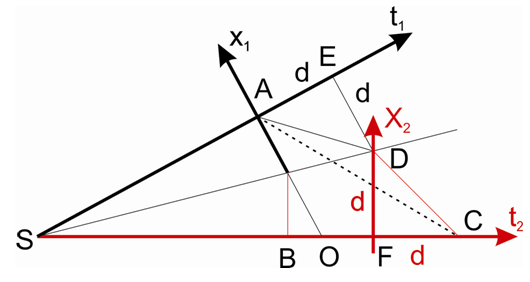 | Figure 3. Suggested mechanism of propagation of EM signals. A signal is sent from point A by a body moving along trajectory t1 and it propagates along direction x1 perpendicular to trajectory t1. It travels distance d along trajectory t1 and distance d along direction x1 (segment AD). In point D quantum is „captured” by a body propagating along trajectory t2 and now it propagates along direction x2 perpendicular to trajectory t2. Now it travels distance d along trajectory t2 and distance d along direction x2 (segment DC) |
5. Interpretation of Results of the MM Interferometer Experiment
Accepting the FER model in which space is absolute is, in a way, a return to the hypothesis of ether [4].The basic argument against the existence of ether was the Michelson Morley experiment. However, in this experiment it was assumed that the motion of quantum and the motion of bodies relative to the medium are the same phenomenon. In the model presented here, the motion of bodies along their trajectories and the motion of quantum are absolute motions relative to the space, but what we observe as motion of bodies of nonzero mass is the result of motion of bodies along the trajectories inclined to each other wherein a measure of the relative velocity is the angle of their inclination. Now, if we consider the MM experiment in the FER, then the motion of quantum and the mirrors’ trajectories are absolute movements, while the interferometer velocity is only the angle of inclination of the trajectories. By changing the velocity of the interferometer we only change the angle of inclination of all trajectories, which does not affect the propagation of signals and the movement of mirrors along their trajectories in relation to each other. The way the MM interferometer works in the FER is shown in Figure 4. | Figure 4. Light propagation in MM interferometer in the FER. The mirrors are in rest relative to each other, so they are moving along parallel trajectories. Light is emitted and reflected at a 45° angle relative to these trajectories, independently of the angle of inclination of trajectories, i.e. velocity equals:. Therefore, the angle of inclination of trajectories of the MM interferometer has no impact on the propagation of light in the interferometer |
As we can see, the present concept of absolute reality - FER- cannot be verified with a MM interferometer. A detailed description of the experiments using the MM and Sagnac interferometers from the point of view of the FER model is presented in [4].
6. Other Problems Related to the Model of Observation Described Above: The Recession of Galaxies and the Shape of Space-Time Interval
The recession of galaxiesOne very strong argument for the method of observing reality proposed here is the phenomenon of the recession of galaxies. Adopting the assumption that we interpret the directions perpendicular to the trajectory of the observed bodies as our space dimensions allows us to instantly explain all the properties of the phenomenon of the recession of galaxies. An example of observation of the recession of galaxies is shown in Fig.5. t = 0 is when the Big Bang - the beginning of the Universe – takes place. Trajectories of all objects in the Universe have their common origin at this point. The observer moves along the trajectory t. Time t0 on the trajectory of the observer corresponds to the age of the Universe because it’s the distance measured along the trajectory (time measured in the observer’s frame) from the Big Bang to the moment of time when the observation is being performed. The observer, located at the point t0, performs the observation of galaxies moving along trajectories t1 and t2. When observing each of the galaxies, the observer interprets different directions in the FER as his space dimensions. In Fig.5, for a galaxy moving along trajectory t1 it is the direction x1, for a galaxy moving along trajectory t2 it is x2. The observer measures the distances from the galaxies along these directions (interpreted by the observer as his space dimensions) and the distances are equal to r1 and r2, respectively.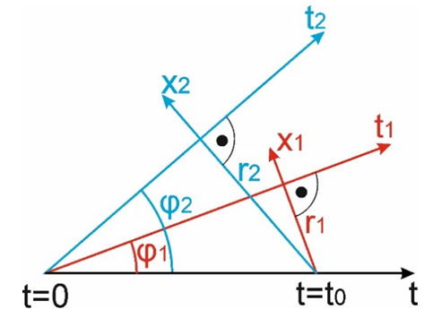 | Figure 5. The recession of galaxies in the FER. An observer and two galaxies move along trajectories with a common origin – the Big Bang. The observer that moves along trajectory t at point t0 observes each of the galaxies along a different direction, perpendicular to the trajectory of an observed galaxy. The distances from galaxies 1 and 2, registered by the observer, are equal to r1 and r2 respectively |
The velocities observed in the observer’s frame using so defined dimensions are equal to: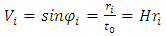 | (5) |
Where i=1,2 – number of the trajectory of the galaxy, t0 – the age of the Universe, H – Hubble’s constant.As one can see, the velocity of the galaxy observed by the observer at point t0 depends on the distance from the galaxy. However, the increase of the velocity with the distance is not the result of any actual acceleration, but is merely a result of performing observations along directions in the FER that are perpendicular to the trajectories of galaxies in the FER and interpreted by observers as their space dimensions. In fact, the galaxies do not accelerate but they move along their trajectories at an absolute velocity equal to 1 relative to the absolute space, exactly like all other bodies in the FER. Therefore, there is no actual acceleration of galaxies and there is no need to search for external solutions like dark energy. At the same time, we have a natural explanation for the value of the Hubble constant as the inverse of the age of the Universe, and from the fact that the observer moves along its trajectory (time axis), it follows that the Hubble constant must decrease with time.Of course, the diagram shown in Figure 5 is simplified because the trajectories of galaxies are presented as straight lines. In practice, the galaxies rotate, perform different motions, so the formula (5) will not accurately describe the speeds of galaxies, but the basic principle is the same, and the fact that the FER model provides such a simple explanation of such a complex problem is one of its major advantages. The same mechanism that leads us to observe the acceleration of galaxies explains the shape of the space-time interval and the time dilation phenomenon.Shape of the space-time intervalLet us consider two observers observing the same body. Since the observer interprets directions perpendicular to the trajectory of the currently observed body as his space-dimensions, then all observers observing this body will interpret the same directions in FER as their space dimensions. An example of several observers observing the same body is shown in Figure 6.We can see that each of the observers sees that the time that passed in the coordinate system of the observed body, i.e. the length of the trajectory of the observed body, can be described in his coordinate system by the following equation (6): | (6) |
where i=1,2 (Fig.6).We can see that the choice of space axes of the observer as perpendicular to the trajectory of the observed body naturally leads to the equation of the space-time interval without the need to define the metric tensor.However, this equation is limited only to cases of observation of bodies. According to the FER model the space-time interval is not an internal property of the reality (the space-time according to TR). It is simply a rule by which we can determine the relationship between the coordinates of observers observing the same body. Such a meaning of the space-time interval is reduced only to the proper time of an observed body and can only have real values. Any conclusions about the consequences of complex solutions of equation (6) cease to make sense. It is easy to guess that the relationship between the observer’s coordinates shown in Fig. 6 will lead to a different transformation of coordinates than the Lorentz transformation and to a different rule of composition of velocity, but it will be described in the following chapters.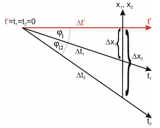 | Figure 6. Two observers moving along trajectories t1 and t2 observe a body moving along trajectory t’. The observers interpret directions perpendicular to trajectory t’ as their space dimensions |
7. Dilation of Time and the Twin Paradox
As it was described above, the observer, while observing the body, interprets directions perpendicular to the trajectory of the observed body as his space-dimensions. The rule of mutual observation of bodies was presented in the previous chapters. We will base our further considerations on Fig. 1. As follows from Fig.1, the observer observing the moving body sees that time in the frame in motion flies slower than in his reference frame – Fig.1a. The situation is symmetrical, because from the frame of the moving observer, a similar time dilation can be observed in its neighbor’s reference frame (Fig.1b). From the geometrical relationships in Fig. 1, one can immediately derive the formulas for the observed dilation of time: | (7a) |
and | (7b) |
However, as we can see, the dilation of time is only an effect of mutual observation and has nothing to do with the actual time dilation we observe - for example in the GPS system.To properly describe actual time dilation, we must make a counterintuitive assumption, which for the time being has to be simply accepted, although explaining it is probably only a matter of time.Let us consider the detector placed in the observer’s frame at the space distance r0 from the origin of the coordinate system. At the time t0 the detector is hit simultaneously by several particles moving at different velocities or, in other words, along trajectories inclined at different angles to the trajectory of the observer.As we can see, the representation of the xyzt point in the observed space-time (Fig.7a) is, in the FER, the sphere with the radius  and with origin in point t0 on the observer’s trajectory (Fig.7b). All points on the sphere must describe the same time – therefore, motion between any two points of the sphere takes no time. If we apply this to our observation we’ll get the situation shown in Fig.8.
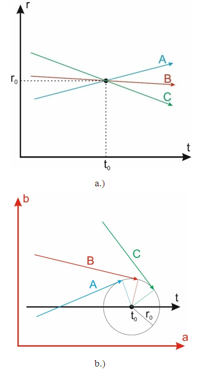 | Figure 7. The point positioned at the time t0 and at the space distance r0 from the origin of the space-time coordinate system -Fig. a - corresponds to the sphere with the radius r0 and center at the point t0 on the trajectory in the FER – Fig. b |
In Fig. 8 we see that as long as both observers are moving along rectilinear trajectories then the effect of time dilation will be symmetrical so that both observers will observe the same slowing of time in the neighbor’s system - exactly as shown in Fig.1. At the moment of the velocity change of, the observer, who changes his speed, travels some part of his route on the surface of the sphere shown in Fig.7b - here the trajectory AB. On the segment AB there is no time flow so the total flow of time in reference frame of body 2 relative to the time flow in the reference frame of body 1 is equal to: | (8) |
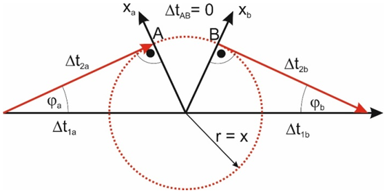 | Figure 8. Twins paradox. Observer 2, when changing his velocity travels some part of his trajectory along arc AB. The time flow between points A and B is equal to zero. Due to the change of the velocity of body 2 from V=sinϕa to V=sinϕb, the observed, mutually symmetrical change of time becomes the actual change of time |
Thus, the change of the speed of the body, whose time in its reference frame is supposed to be shorter, is a necessary condition for changing the observed symmetrical dilation of time of one body relative to another into the actual change of time in the frame of the body whose speed has changed. Hence, the time dilation in the frame in motion is not only the result of velocity but, primarily, the result of the change of the velocity. However, the resulting formula is the only a function of velocity, which has been a source of misunderstandings for many years [1, 2]. Therefore, the time dilation resulting from the motion of satellites of the GPS system requires the change of direction or value of the velocity and it is only under this condition that the formula describing the time dilation, nota bene identical as the one derived from the Special Theory of Relativity (1), properly describes the indications of the satellite’s clock. More about the physics of the time dilation can be found in the chapter “Example: The quantized time dilation in case of twin paradox”.
8. Transformation of Coordinates versus the Lorentz Transformation
In the chapter “Form of the space-time interval” I have shown how the shape of the space-time interval can be obtained. At the same time, the problem of observation of a body by several observers, shown in Fig.6, allows to find the transformation between coordinate systems of observers of the same body. From simple geometric transformations resulting from Fig.6 one can obtain formulas for transformation of coordinates which also satisfies the equation of space-time interval; however, it differs from the Lorentz transformation. The new transformation formulas take the following form: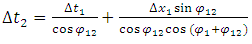 | (9) |
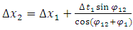 | (10) |
where:The velocity of observer 1 relative to observer 2 is: | (11) |
whereas the velocity of the body observed by the two observers (moving along trajectory t’ in Fig.6) relative to observer 1 is: | (12) |
The time dilation formula resulting from formula (7) is no different from the analogous formula resulting from the Lorentz transformation: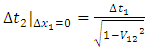 | (13) |
while the relativistic length contraction, according to formula (8) should not take place: | (14) |
Thus, the proposed approach explains the observed dilation of time in reference frames in motion, while also explaining the failure in proving the relativistic length contraction.According to the proposed model, the Lorentz transformation is mathematically correct but non-physical, because the two equations of Lorentz transformation describe two different bodies moving along different trajectories, and both equations have a common solution only at the point of intersection of these trajectories. The exact explanation of this problem and the extended form of formulas (9) and (10) are available in [5].
9. Composition of Velocities and Proposal of Experimental Test Confirming the New Approach
The new transformation of coordinates leads to the new rule of composition of velocities. Since velocity is a function of an angle between trajectories, the composition of velocities relies on the addition of angles, according to Figure 6. If the angle between the trajectory t' and t1 is ϕ1 and the angle between the trajectories t1 and t2 is equal to ϕ12 then the velocity of the body traveling along the trajectory t’ relative to body traveling along trajectory t2 is: | (15) |
which, rewritten using velocities described by the formulas (11) and (12), takes the following form: | (16) |
A similar relationship was also derived by another author using a different method [6].A comparison of rules of composition of velocities for two identical velocities for Galilean and Lorentz transformations and according to the FER model presented here is shown in Fig. 9.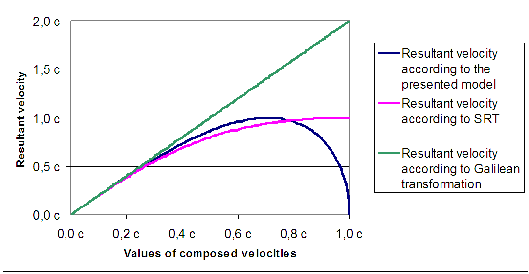 | Figure 9. Composition of two identical velocities according to Galilean and Lorentz transformations and according to the FER model presented here |
According to formula (16), we still cannot exceed the speed of light, but by composing the appropriate velocities we can reach a 90° angle between the trajectories, which corresponds to the speed of light (Fig.9). This should lead to registering experimental results. A proposal of such an experiment for obtaining measurements of total proton-proton cross-sections [7] shows that in the case of two colliding beams we should observe doubling of total cross-section for the energy of each of colliding beams corresponding to the velocity of each beam V = sin (45°). When these speeds are exceeded, a discrepancy between the total cross section for collisions of fast protons with the stationary protons, with analogous experiments using two colliding beams of the same relative velocity resulting from the Lorentz transformation, should occur. The occurrence of such discrepancies in measurements of cross section for high energy protons of cosmic origin with the protons in the atmosphere was previously described in [8].However, the following question may be asked: if for the colliding beams of energies corresponding to velocity V = sin (45°) for each beam, there should occur a clear difference between experimental results and the predictions of TR and the difference occurs for the values of energy achieved in typical experimental devices, why has no one observed such effects so far?According to the calculations from [7], such anomalies occur only in a very narrow energy range and require very homogeneous energy of beams. For example, for this experiment with total proton-proton cross-section measurements, with a proton beam’s energy of about 0.4 GeV, proton energies should match the desired energy to the up to several hundred eV. Greater width of distribution of energy will result in detecting only a slightest increase in statistical errors at this energy.Similarly as in the described experiment, it should be possible to observe the anomalies in a strictly defined energy range in other experimental devices as well, but it requires very narrow energy distribution of the colliding beams.
10. Description of Phenomena in FER and Description of Phenomena in Relativity Theory - Summary and Introduction of Complex Notation
In Theory of Relativity it was assumed that the reality surrounding us is built of three space dimensions and one time dimension. Phenomena were therefore described as functions of space-time dimensions. However, the equations of TR describe the variability of these phenomena not with respect to these coordinates but with respect to three space dimensions and a space-time interval - instead of the dimension of time.In the FER, we assume that there are four identical dimensions abcd creating the Euclidean space (space, not space-time, because the ideas of time and space refer to the perception of dimensions abcd through the observation of bodies in that space and they are a property of observation rather than the dimensions of reality). All phenomena are functions of these four dimensions, and their variability is also related to these dimensions and not to any other values, that are not the dimensions of reality - as it was done in the case of TR. In practice, when describing the motion of a body in FER, we do not have to use the dimensions abcd of which the FER is composed. We can use any orthogonal coordinate system - for example, a coordinate system consisting of the time axis of the reference system of observed body - t' (trajectory of observed body in FER) and the three space-dimensions of the observer of this body (perpendicular to the trajectory of the observed body). It is a coordinate system of four orthogonal directions in FER so we can use it to describe phenomena, because there is no distinguished direction in space in FER that would force the selection of a set of orthogonal directions to describe phenomena.Therefore, when describing events in FER we can, similarly as in TR, relate the variability of phenomena to the spatial coordinates of the observer and proper time of the observed body - which is, in the case of observation of a specified body, the space-time interval, but unlike in TR, the phenomena are also functions of the same coordinates - xyzt' instead of xyzt. A similar approach has been previously suggested in literature attempting to describe the reality with the help of Euclidean model, e.g. in [9-11]. However, the fundamental difference between the use of xyzt’ coordinates to describe reality in previous works and the FER model presented here is that in those works the xyz coordinates (t' was individually chosen) were a part of the reality (objective dimensions creating reality) so they were common for all bodies, while according to the FER model, the only common dimensions are abcd, whereas the FER directions interpreted as xyzt' dimensions are chosen individually for each observed body. In other words, for each case of observation, the dimensions of xyzt' are orthogonal to each other but they are rotated in FER in relation to the directions xyzt' describing another observed body. And this difference in the orientation of the xyzt’ dimensions relative to the orientation of the dimensions of other bodies is the sole source of the relativistic effects in uniform rectilinear motion.If we describe phenomena as functions of the observed body's proper time and space dimensions of the observer, it is convenient to use complex notation to separate the phenomena that are the function of the absolute motion of the body along its trajectory from the phenomena associated with the relative motion of the bodies and the exchange of interactions along three spatial directions. We use this complex notation here in an unusual way, because we assume one dimension to be imaginary and the other three to be real. The imaginary direction is not the property of space but merely the property of observation. It means that by describing the observation of a body we describe its trajectory as an imaginary direction - only for the purpose of describing the observation of that particular body. For phenomena with spherical symmetry in space, the following description of coordinates can be used: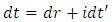 | (17) |
where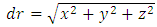 | (18) |
So, in very general terms, if the observer during observation travels the distance dt along his trajectory, then in relation to the observed body he will travel a distance dr along directions interpreted by him as space dimensions, where the distance dr is defined by the formula (18), and the distance dt’ along imaginary direction determined by the proper time of the observed body.By calculating the module of so defined distance (17), we will obtain the equation of space-time interval for the case of observation of a particular body - formula (6). Thus, introducing covariant notation is no longer necessary.
11. Wave Structure of Particles and Description of Quantum Mechanics Phenomena
If particles move at constant velocity with respect to the absolute medium - FER – then we no longer have any obstacles to describing the particle directly as a wave propagating in the elastic medium; thus the FER can now be considered as such. The amplitude of the wave should disappear at infinite distance measured along the direction perpendicular to the trajectory of the particle/wave and it should have a frequency calculated from the dependence | (19) |
I’m going to suggest the following formula describing the wave corresponding to this particle: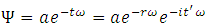 | (20) |
where a – the amplitude of wavet – the observer’s time described with the formula (17).Wave is a function of the position of the particle on its trajectory in FER. If we want to describe this function as a function of the space-time coordinates (xyzt) of an observer then we can use the following relationship: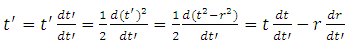 | (21) |
Substituting (19) and (21) in the formula describing the wave in FER (20) we obtain: | (22) |
As we can see, the wave defined in the FER with the formula (20) after transformation to space-time coordinate system takes form of a well-known wave function, which is a solution of the Schrödinger equation, multiplied by the segment describing the amplitude distribution as a function of the distance from the particle (22). While the wave function in formula (22) is not directly measurable in the “classical” space-time, the corresponding wave in FER described by formula (20) describes the real deformation in the FER. So, the abstract wave functions known from the currently used model correspond to waves in FER. Instead of using complex and abstract tools of Quantum Mechanics we can solve problems of particles/waves interaction by examining the interactions of waves representing the particles in the FER, which can be treated here as an elastic medium in which the interactions propagate. The tools to solve these problems will be simpler and more intuitive than the analogous tools provided by Quantum Mechanics. Many of the problems that appear in Quantum Mechanics can be explained and described by the FER model in a much simpler way than in QM and the new approach can explain some enigmatic properties of particles.Let us start by looking at the function describing a particle as a wave in FER, using the form proposed by equation (20).The function can be written as follows: | (23) |
Bearing in mind that imaginary values refer to the direction determined by the trajectory of the observed body, we see that the equation (23), describing a particle, describes transverse oscillations perpendicular to the trajectory of the particle (the real values) and longitudinal oscillations along the trajectory of the particle (the imaginary values). It is clear that the equation describing a particle in practice does not describe the vibrations but the rotation (or superposition of rotations) in plane (planes) formed by directions perpendicular to the trajectory of the particle and the direction determined by the particle’s trajectory. The amplitude of the oscillation is here at the same time the radius of rotation with the center in the center of the particle/wave. At the present stage a model of such a particle is not yet complete, but the fact that what we observe or interpret as waves is in practice the rotation, and the waves observed by us are only projections of this rotational movement on the directions interpreted by us as spatial dimensions, allows us to explain, in a trivially simple way, such properties of particle/wave as, for example, the spin.If we use the formula for the angular momentum of the rigid body: | (24) |
then for a particle with the wave frequency described by the formula (19), the formula for the angular momentum takes the following form: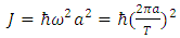 | (25) |
Where T – period of oscillation of the particle/wave.If we now assume that the velocity of rotation in the plane, e.g. xt', is | (26) |
then it follows that the angular momentum of a given particle is: | (27) |
and it is directed along one of the space-dimensions. Thus, by registering a particle in the space-time, we observe it as a particle, described by a wave function that has an angular momentum. Such angular momentum does not have to be considered a mysterious property of particles - in this case, the angular momentum is a result of the actual rotation of the body/wave. The actual value of the angular momentum of the particle will be different than the one given in (27) - the particle structure may differ from the model shown here: the rotations may occur in differently oriented planes, the particle/wave may be a superposition of various waves, etc. This problem has not been sufficiently analyzed yet; however, as we can see, the model offers ways to obtain various solutions which will hopefully be consistent with the actual state of knowledge.
12. Waves of Matter and the Time Flow
The representation of a body directly as a wave, with the wavelength/(period of oscillations) of the waves of matter (not in the sense of the de Broglie waves of matter; the problem will be described in more detail below) defined by the formula (19), propagating along one of the directions in the FER interpreted by the body as its time-dimension, gives a different view on the problem of time. By measuring time in everyday life or in laboratories, we always use oscillations - from the oscillation of the pendulum of the clock to atomic oscillations. In the case of presenting a particle as a wave, i.e. as oscillations of a medium, it is natural for the body to accept the number of oscillations as a measure of the particle’s proper time. So, if the wavelength (or period of oscillations) of particle/wave is equal to T then the particle's proper time can be represented as multiples of the periods of oscillations of the particle/wave | (28) |
Since all trajectories are equivalent, identical particles moving along different rectilinear trajectories have identical periods and amplitudes of oscillations.The measure of the time that flows in the particle’s system will not be the length of the trajectory traveled by that body in the FER but the number of the particle/wave oscillations on the route between the two points in the FER.In this way, the definition of a particle as a wave naturally introduces the quantization of time, which is no longer a continuous but a discrete value - measured by the number of periods of body’s waves. The quantum of time for a given particle will be the period of oscillations of waves of matter defined by the formula (19).I will remind you that in addition to the time we perceive, which is measured by the number of particle/wave oscillations, absolute time is also introduced in the FER model. In practice, the absolute time corresponds to the distance traveled between two FER points, and for all bodies traveling between these points, the absolute time flow is identical. On the other hand, the number of oscillations – i.e. the measure of the proper time of the body - is different for each body and depends on the trajectory along which the body crossed that distance. A little more about this in the next chapter.Example: The quantized time dilation in case of twin paradoxThe rule of observation of the relative time dilation was shown previously in Fig.1. The same situation for two identical particles/waves (with identical vibration periods) is shown in Fig.10.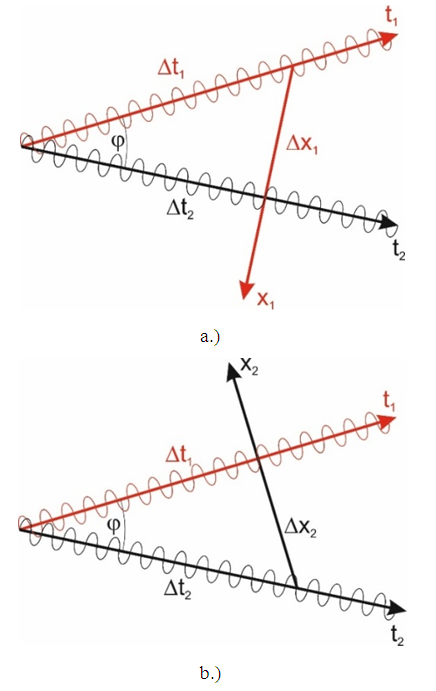 | Figure 10. The situation is identical to that shown in Fig.1, however, the proper times of the reference frames of bodies are not expressed by the length of the trajectory but by the number of oscillations. For two identical bodies, the number of oscillations per unit of length of the trajectory is identical for both bodies. The observed time difference is the result of interpreting a direction perpendicular to the trajectory of the observed body as the space-dimension of the observer’s coordinate system |
Now, we can rewrite formulas (7) for the observed time dilation, for the case of quantized time, where the quantum of time is the period of body’s oscillation/wavelength equal to T. Then the times of bodies can be written in the following form: | (29) |
 | (30) |
where  is the number defining the time flow in the reference frame of observer "i" with the help of number of wave’s oscillation periods.In this case, the observed dilation of time can be writtenfrom point of view of observer 1:
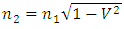 | (31) |
from point of view of observer 2: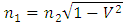 | (32) |
Now, analogously to the description of the twin paradox presented in the chapter “Dilation of time and the twin paradox”, we can present the problem from Fig.8 with the help of time expressed by the number of periods of oscillations of particles - Fig. 11. As we can see, in the case of infinite acceleration corresponding to the movement of the particle from point A to point B in Fig.11, the oscillations of particle do not take place - so the time flowing in the reference frame of the particle is equal to zero for the arc AB. Thus, the time flowing in the reference frame of body 2, measured by the number of oscillations, will be shorter than the time in the reference frame of body 1.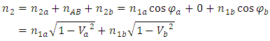 | (33) |
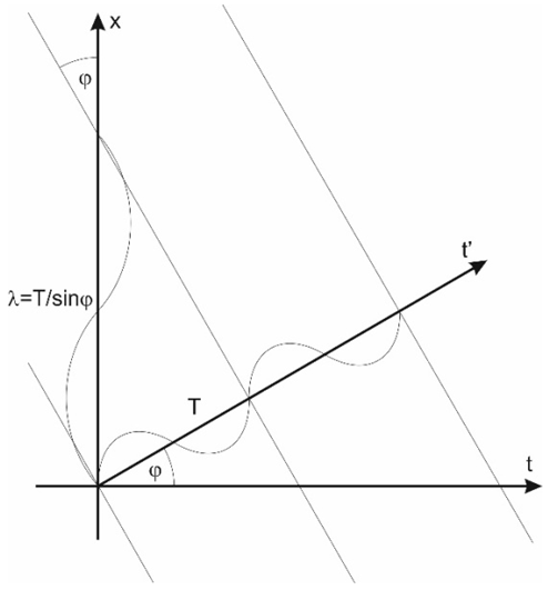
In practice, for non-inertial motions - as a conclusion from the Fig.11 - one should expect a decrease in the number of oscillations and extension of periods of oscillation along curved trajectories. And it is this extension of the periods of oscillations for the curved trajectory that is responsible for observing the dilation of time (lower number of oscillations) in the reference frames of the GPS system satellites or in the Hafele-Keating experiment [1, 2] (I am not taking into account the gravitational change of time here). In other experiments confirming the dilation of time phenomena, the most important factor determining the value of the time dilation is the change of velocity as shown in Fig.11, while the oscillation periods of the body do not change. Meanwhile, according to the TR, in all the cases described above, the time dilation is the result only of the linear velocity of the bodies. The extension of the oscillation period as a result of changing the direction of body/wave propagation (motion) in the FER is not yet completely explained and mathematically described. It will most likely be connected with the nature of the oscillations and with behavior of these oscillations when changing the direction of propagation of the oscillations - especially since the particle described by wave according to equation (20) is not limited to specific dimensions in space but it extends to infinity, so any change of direction will disturb the shape of the wave up to infinity, which will have to lead to the changing of the wave’s oscillation period of at different distances from the center of the body/wave. The illustration of this predicted mechanism is shown in Fig. 12. It probably results from the fact that in the region where the oscillation period ”T” is shorter (in Fig. 12 b the region below the segment AB), the energy of wave (described with the formula: E=h/T) increases, while in the region where the oscillation period is longer (in Fig 12 b the region over the segment AB), the energy of the wave decreases; this will result in shifting the center of the wave to the region of lower energies with longer oscillation periods. As we can see, the change of direction of motion of the wave in the four-dimensional space should cause deformation of the waves, which on the one hand causes the effect of time dilation, but on the other hand it must also cause tensions in the medium, therefore the change of direction of body/wave must be related to the occurrence of forces which we probably recognize as forces of inertia. Thus, the mechanism proposed in Fig. 12b most probably justifies the time dilation as well as the inertial forces and, in a simple way, shows the relationship between these two phenomena. The problem of mathematical description remains open, but the main idea is defined here and, in my opinion, finding a mathematical description of the oscillation - or rather the rotation of a medium - following the already known laws concerning such dilation of time and inertial forces is only a matter of time.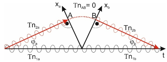 | Figure 11. The situation is identical to that shown in Figure 8, but here the time is presented as the number of body/wave oscillations. There are no oscillations along the AB curve, hence the time (number of oscillations) of body 2 is shorter than the time (number of oscillations) of body 1 |
 | Figure 12. A wave propagating along a straight line is shown in Fig.a. In Fig.b, the same wave is propagating along a curve. The dots show the maximum amplitude of the wave. The AB distances on both drawings are identical but the time in the particle’s system, measured by the number of oscillations, is shorter in the reference system of a particle propagating along the arc. In Fig.a time is equal to 9 periods while in Fig.b - to 7 periods |
We can see that the mechanism of the time flow in the body’s reference frame in motion is defined by the number of oscillations of the period, which in the case of inertial movements is constant while it is extended in the case of non-inertial motions. The decrease in the number of oscillations caused by the change in direction of velocity (Fig. 11) or caused by the change in the period of oscillations (Fig. 12) is detected as the time dilation.
13. Energy of Particles and Energy of Macroscopic Bodies
If we consider the energy of macroscopic bodies it is easy to guess that if we want to obtain the known relationship between momentum, energy and the rest mass of the observed body (here equal to its rest energy), energy and momentum can be presented in the FER as vectors overlapping the trajectory of the observed body and the coordinates of the observer ‘s coordinate system, as shown in Fig.13.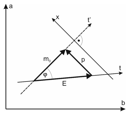 | Figure 13. Diagram showing the relation between energy, momentum and rest energy (mass) of a body in the FER. The observed body moves along trajectory t’, an observer along trajectory t |
Thus, the body’s energy observed in the observer’s reference frame relates to the rest energy of the body similarly to the relations between times of the observer and the observed body (7):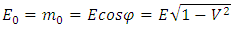 | (34) |
If we now consider a particle as a wave - according to Fig.10 - we observe the change of time, but this change of time is related to the number of oscillations with a fixed period rather than to the change in observed oscillation period. If a similar relation to (34) is to occur for the energy of the wave of matter defined by the formula | (35) |
then the observer must observe not the change in the number of oscillations but a change in the wavelength/oscillation period (these two concepts are, in the FER, equivalent) of the wave of matter.If in case of motions of macroscopic objects we have chosen the directions perpendicular to the trajectory of an observed body as the space axes of the observer, then in case of interference of waves responsible (according to the FER model) for the occurrence of quantum effects, we will have to adopt another approach.If the dependence (34) is to be conserved, then for a wave moving relative to the observer’s coordinate system, the space dimensions of the observer’s coordinate system should be perpendicular to the trajectory of the observer, and not to the trajectory of the observed body, as in the case of macroscopic motions. The described situation is illustrated in Fig. 14. The reasons such a mechanism needs to be applied here still require a proper explanation, but for now, in order to preserve the coherency of the model, we need to accept such an assumption. Therefore, for all further considerations regarding direct interactions of/with the waves of matter, we are going to use coordinate systems in which the space directions are perpendicular to the time axis of an observer. | Figure 14. In case of direct interactions of bodies/waves (interference), we describe the energy of the body/wave in the observer's rest frame (the observer's spatial axis is perpendicular to the observer's trajectory) |
In this case, we can describe the particle’s energy as follows:The rest energy of observed particle | (36) |
The energy of a particle in the observer’s frame according to Fig. 14 can be expressed with the formula: | (37) |
We should remember that the direction in the FER that we interpret as a space dimension is not constant but depends on the way of performing the observation or, in other words, from the manner in which the interactions are exchanged. The exact interpretation of the situation shown in Figure 14 needs to be developed further; however, accepting such a description allows to bind the wave character of particle described above with the relativistic dependences between motion and energy in macroscopic cases.At the same time, it should be noted that to determine the energy of a particle/wave we must know its trajectory in FER, because the energy is defined by the angle between the trajectories of the particle and the observer (37). For this we must observe at least one full cycle - equal to the period of oscillation.Thus, the observation time t must be longer than the wave/particle period:  , and because
  , the following dependence must be satisfied:
 | (38) |
This is the property that results directly from the wave nature of the particle and from the fact that the energy (velocity) can be determined by knowing the angle of inclination of trajectory of the observed body to the observer’s trajectory.Too short time of measurement- shorter than the period of wave/particle oscillation - results in a less accurate determination of trajectory and hence of the energy of particle.
14. Momentum of Particles/Waves Versus Momentum of Macroscopic Particles
If we are using a unit system in which c = 1, then, according to the situation shown in Fig. 13, the momentum of the particle should be defined by the relation: | (39) |
which in the case of non-relativistic particles, with which we deal in typical experiments and applications, may be written as: | (40) |
Where the observed wavelength λ is equal to: | (41) |
The wavelength λ described with the formula (41) is already known as the de Broglie waves of matter. According to the FER model the de Broglie waves of matter are the intersection of the surfaces of constant phases of the waves of matter described by formulas (19) and (20) with the space-dimensions of the observer’s reference frame, as shown in Fig. 15. If we want to measure the momentum and position of the particle/wave then from the fact that to determine the trajectory, the time of measurement must be greater than the oscillation period, it follows that the observed distance in the xyz space must be greater than or
or  which means that if
  then:
then: | (42) |
 | Figure 15. The intersection of the surfaces of constant phases of the waves of matter of observed body with the spatial dimensions of the observer's system gives the de Broglie waves of matter, the length of which is a function of velocity, and therefore also a function of momentum, of the particle/wave |
So, according to the formulas (38) and (42), analogous to Heisenberg's inequality, if we are considering the particle/wave, then defining the trajectory along which this wave propagates requires measurements that take into account the distance equal to or greatfer than the wavelength of this wave, because for shorter distances we are not able to determine its trajectory with sufficient accuracy.
15. Particle Size, Probability, Particle Diffraction on the Slit
As shown above, while analyzing the wave/particle structure we deal with several values. For the time being, we will be using these values to describe an electron. They are only an example, because if the distribution of the amplitude of the electron’s wave differs from the distribution given for the simple wave described above (20), then these values will also vary.1. The radius “a” in the formulas (20), (23), in the case of a projection of rotation on space-dimensions, is the amplitude of oscillations. For an electron, the amplitude "a" is equal to approx. 4E-13m (computed on the base of formulas (19) and (26)).2. If we substitute the values corresponding to this amplitude to the formula (20) determining the amplitude of the wave as a function of distance, we will get the width of the amplitude distribution at mid-height of about 4E-20m. This distribution was chosen as the simplest one for the purposes of the description, but it is expected that the shape of amplitude will differ from the one assumed in formula (20).3. If we calculate the length/period of the electron wave from the dependence  for FER where c=1, then the length of the wave of matter will be equal to 2,5E12m – that is, equal to the circumference of the circle defined by the radius “a” calculated in point 1 (from the condition that the linear velocity on a circle of radius a is equal to 1).Note that the particle’s size measured along the direction perpendicular to the particle’s trajectory, for the case of an electron, is about 4E-20m while the wavelength of matter is approximately. λ0=2,5E-12m. These dimensions will allow us to determine the behavior of an electron on a slit.Let consider a two-dimensional plane on which we have a designated slit and an electron’s trajectory perpendicular to the slit. The observer's time axis is perpendicular to this plane – Fig.16a. The particle is shown as a wave. In the case of the three-dimensional space shown in Fig.16, we have two directions interpreted as space dimensions - xy - and the third direction interpreted as time-dimension. As the time axis, we took the trajectory of the slit in the graph. The particle’s trajectory is inclined to the slit trajectory at an angle ϕ, so the particle’s velocity relative to the slit is
  – Fig.16b.In the 3-dimensional case presented on the diagram, the surfaces of the constant phase for the wave are planes perpendicular to the trajectory of the particle. The wavelength of matter determined from the formula E=hν is equal to the wave’s oscillation period T. The projection of a surface of constant phase of a wave on the XY plane gives the de Broglie waves with wavelength λ=T/sinϕ on the plane XY (Fig. 16 b, 17, formula (41)).
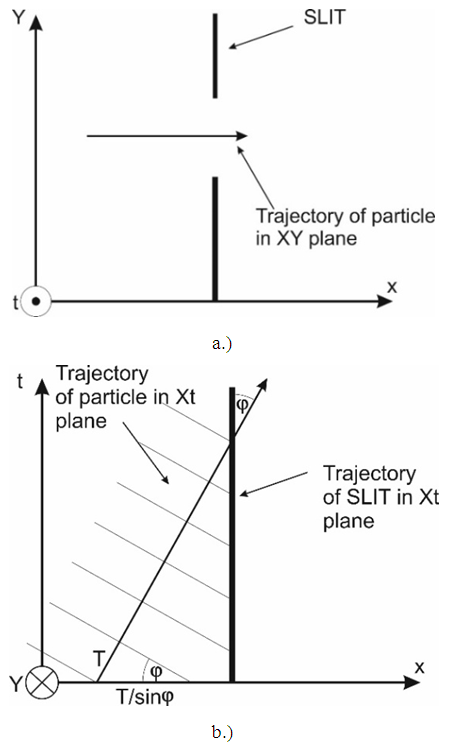 | Figure 16. A particle/wave passing through a slit. Fig. a shows the view in the xy plane, in Fig. B, the view in the xt plane. The time axis is chosen as parallel to the trajectory of the slit. Projection of the wavelength T of matter on the xy plane (fig. b) is the de Broglie’s wave of matter - identical like in Fig.15 |
It should be noted that while the wavelength observed in our space depends on the momentum of the particle, the particle size measured along the direction perpendicular to the particle’s trajectory resulting from the wave amplitude distribution is constant and many orders of magnitude smaller than the wavelength of the particle in space (see point 2 above). This means that if a particle falls on a slit, the diffraction result is determined by two factors - the de Broglie wavelength of the particle resulting from the momentum of the particle, and the location of the maximum amplitude of particle/wave relative to the slit.The described situation is shown in Fig.17, where the dot indicates the area of maximum amplitude (which, as I wrote above, is many orders of magnitude smaller than the wavelength, and therefore also smaller than the size of the gap which in Fig.17 is comparable to wavelength). Changing the position of the maximum amplitude relative to the slit will result in different intensity distributions of the diffraction image for single particles (Fig. 17a and 17b). It has nothing to do with the probability being some mysterious feature of a particle. This is simply a result of the structure of particle treated as a wave in FER.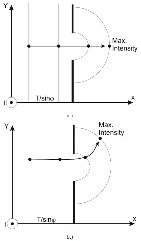 | Figure 17. The dependence of image behind the slit for the particle passing through the slit as shown in Fig.16 from the position of the maximum amplitude relative to the slit. In Fig.16a, the maximum amplitude of the particle is in the center of the slit, in Fig.16b, the maximum amplitude of particle is shifted towards the edge of the slit |
16. Particles and Fields
The described particle model as a wave in a medium such as FER allows for a different look on the problem of fields and particles. The wave amplitude distribution given in formula (20) was chosen at random and would most likely have to be adjusted to the actual particle properties. However, according to amplitude distribution, a small portion of the particle appears to be a region with an amplitude much larger than in the rest of the region, but the disturbance of space extends to infinity. It means that it will probably be possible to describe the entire wave as roughly divided into two areas: the center of the wave treated as a particle, and the remote region treated as a field. Particles, even very distant, can interact with each other through the space disturbances that they generate, and the space, as one can expect, should affect the particle system in a way that decreases the total energy of the system. Such interaction should have the properties of a field. At this stage, it is only a concept not yet supported by calculations, but it is to be expected that we will be able to find such amplitude distribution and the parameters of the space treated as a kind of elastic medium that the interactions between the waves at long distances will have the properties of fields.If we treat the FER as an elastic medium, the energy of oscillation of this medium for slight deformation in the case of oscillation in one direction should be proportional to the square of amplitude of oscillations. In the case of a particle described as a wave, the energy is determined by the formula | (43) |
If we use the formula for the fine-structure constant, then in the unit system where c = 1, the energy equation will take the following form: | (44) |
Thus, according to the formula (44), if FER is assumed to be an elastic medium, the value of the electrical charge should be related to the deformation of the medium - compression or stretching. Compression or stretching of the space would probably determine in this case the sign of the electric charge. We therefore have a proposal of the concept of electric charge treated as deformation of space. This is a suggestion indirectly based on the assumptions of the model. Time will tell if this suggestion is justified.
17. Conclusions
The idea of a new description of reality presented here is based on accepting a model of reality in which the "true" reality is as simple as possible, while our perception makes us interpret different directions in this space as our space-time dimensions. Directions interpreted as space-time dimensions are not the objective properties of reality but depend on the bodies currently observed. This is logical because we learn about the existence of space, the number and structure of dimensions, indirectly - through observation of the surrounding particles. The idea to bind the space-dimension of the observer not to the space but to the currently observed body allowed to achieve a much simpler description of the relativistic phenomena and allowed to explain, within a single model, many of the phenomena which have so far been described with different models. For instance, the mechanism mentioned above explains the limitation of the speed value to the speed of light, the constancy of the speed of light, the time dilation, the phenomenon of the recession of galaxies, and removes the singularities occurring in the previous models. At the same time, the interpretation of the relative motion of the body as an angle of inclination between the trajectories in absolute space allows to connect the absolute movement of particles relative to FER along their trajectories (time flow) with the relative motion of bodies (angle between trajectories), explains the Mach principle, and allows to describe the particle directly as a wave, to which the projection on observed space-time (xyzt) gives the wave function.Moreover, the description of the particle as a wave allows to connect Quantum Mechanics with the phenomena described so far by the Theory of Relativity, explain the quantum nature of time in a simple way, gives a simple interpretation of Heisenberg’s uncertainty principle, and gives the basis for unifying description of particle and field. Simultaneously, the conclusions allow a simple interpretation of the electric charge as deformation of space. The proposed approach is not complete yet. Not all ideas have been described mathematically. However, all the ideas and conclusions described here make a coherent and closed model in which all elements support each other. The issue of mathematical description of many phenomena is open, but it is only a matter of solving the problems unambiguously defined in this work.In this paper, I am proposing a new model of reality. This model still requires a lot of work, such as finding the particle amplitude distribution, specifying the properties of space, describing wave interactions in a way that explains the EM fields and gravity. On the other hand, accepting a new model will result in changing the mathematical apparatus used to describe reality. There will be no need for covariant notation or for the use of operators used in TR and QM up until now. Of course, TR and QM tools can still be used for many years to describe physical phenomena, but one needs to be aware that the range of phenomena described by these tools will be limited and not as broad as the description proposed by the new model. Accordingly, the description of the reality proposed in this paper may not be accepted by many physicists accustomed to the tools already used to describe reality. However, I hope that, even though adopting a new model may lead to students knowing more about a new theory than their professors for a while, the theory will be taken seriously and at least tested experimentally [7], which is currently possible with the use of available experimental systems and diagnostic tools.
References
| [1] | W. Nawrot "The Hafele and Keating Paradox" - Phys. Ess. 17, 518 (2004). |
| [2] | W. Nawrot, "The Hafele-Keating paradox - Serious problems of the special theory of relativity (SRT)?" Phys. Ess. 27, 4, pp 598-600 (2014). |
| [3] | W. Nawrot "Proposal of simpler description of SRT" - Galilean Electrodynamics 18, 43-48 (2007). |
| [4] | W. Nawrot, "New philosophy of Aether in Euclidean Reality model and interpretation of indications of Sagnac and MM interferometers" Proceedings of the 20 NPA Minneapolis, MN USA 2013. |
| [5] | W. Nawrot "Is the Lorentz Transformation a physically correct solution of the space-time interval equation?" - Galilean Electrodynamics Vol. 20, Special Issue 2, 34-37 (2009). |
| [6] | Rob van Linden, “Dimensions in Special Relativity Theory”, Galilean Electrodynamics 18, 12-18 (2007). |
| [7] | W. Nawrot, "Proposal of experiment disproving the Theory of Relativity" Accepted for publication in the Galilean Electrodynamics. Available at http://euclideanreality.com/pdf/DisproofOfSTR.pdf. |
| [8] | J. Velasco, J. Perez-Peraza, A. Gallegos-Cruz, M. Alvarez-Madrigal, A. Faus-Golfe, A. Sanchez-Hertz, “σpptot Estimations At Very High Energies” arXiv: hep-ph/9910484v1 (1999). |
| [9] | Hans Montanus “Special relativity in an absolute Euclidean Space-Time” (Physics Essays, vol. 4, nr 3, 1991). |
| [10] | Jose Almeida “An alternative to Minkowski space-time” (arXiv:gr-qc/0104029, 2001) |
| [11] | Giorgio Fontana “The Four Space-times Model of Reality” (arXiv.org, physics/0410054A). |
| [12] | W. Nawrot "The structure of time and the wave structure of the matter" - Galilean Electrodynamics 18, 49-53, (2007). |
| [13] | W. Nawrot "Four-Dimensional Euclidean Reality - The basic properties of the model" Proc. International Scientific Congress "Fundamental Problems of Natural Science and Engineering" Saint-Petersburg, Russia 2008. |
| [14] | W. Nawrot "Euclidean Reality Theory - Spectacular Conclusions and New Problems" - Proc. International Scientific Congress "Fundamental Problems of Natural Science and Engineering" Saint-Petersburg, Russia 2008. |
| [15] | W. Nawrot "Recession of galaxies, simpler explanation" - Galilean Electrodynamics Vol 20, Special Issue 2, 38-40 (2009). |
| [16] | W. Nawrot, "Euclidean model of the space-time - is the reality exactly as we can observe it?" - Mathematics, Physics and Philosophy in the Interpretations of Relativity Theory, Budapest, 4 - 6 September 2009. |
| [17] | W. Nawrot, "Explanation of twin paradox according to the Euclidean Reality Model" Proceedings of the 20 NPA Minneapolis, MN USA 2013. |

 Abstract
 Reference
 Full-Text PDF
 Full-text HTML