Bratianu Daniel
Str. Teiului Nr. 16, Ploiesti, Romania
Correspondence to: Bratianu Daniel, Str. Teiului Nr. 16, Ploiesti, Romania.
| Email: |  |
Copyright © 2017 Scientific & Academic Publishing. All Rights Reserved.
This work is licensed under the Creative Commons Attribution International License (CC BY).
http://creativecommons.org/licenses/by/4.0/

Abstract
According to general relativity, the gravity is a property of the curvature of space-time. A curved 3-dimensional space is also considered to be equivalent to a gravitational field. On the basis of this assumption, a connection between the curvature of 3-dimensional space and stationary electric currents is found. Starting from this connection, a relation between the metric of 3-dimensional space and magnetic vector potential is established. Several applications are given.
Keywords:
Weyl vector, Weyl connection, Magnetic field, Stationary electric currents, Long straight wire currying current, Helical motion
Cite this paper: Bratianu Daniel, Magnetostatics and Gravity, International Journal of Theoretical and Mathematical Physics, Vol. 7 No. 4, 2017, pp. 90-94. doi: 10.5923/j.ijtmp.20170704.03.
1. Introduction
According to GR, the gravity is a curvature of space-time. We consider that the same is true for the 3-dimensional space, so that, without gravity, the 3-dimensional space possesses Euclidean geometry, and the curvature tensor is identically zero. Also, according to GR, a measure of the curvature of space-time is given by Riemann-Christoffel curvature tensor. Again, we consider that the same is true for the 3-dimensional space. So, let us consider a 3-dimensional space, equipped with a Riemannian metric  | (1) |
that is conformal to the Euclidean metric  | (2) |
where  is the Kronecker symbol
 and
and  is a function of the Cartesian coordinates
 Therefore, as in [1] the metric tensor of such a metric is given by
 | (3) |
2. The Field Equations
Starting from the metric of space (1), we can deduce the well-known RC curvature tensor, as in [2]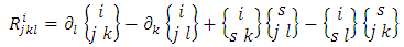 | (4) |
where the symbol  means partial derivative with respect to
  , and the quantities in brackets are Christoffel symbols of the second kind, or what we call the Levi-Civita connection
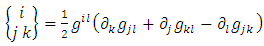 | (5) |
Substituting now (3) into (5), the Levi-Civita connection becomes the Weyl conformal connection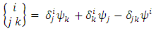 | (6) |
where we introduced the notations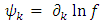 | (7) |
 | (7a) |
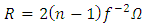
for the components of Weyl vector. From the RC curvature tensor (4), we can get the well-known contractions. First is the symmetric Ricci tensor  | (8) |
and the other is the scalar curvature | (9) |
Therefore, we can build the well-known Einstein field equations, as in [3]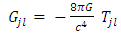 | (10) |
where we consider that  is the energy density tensor of the gravitational field, and
  is the well-known Einstein tensor
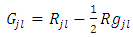 | (10a) |
From the Bianchi identities,  | (11) |
where the symbol  represents the covariant derivative with respect to
  , we deduce that the covariant divergence of the energy density tensor is identically zero
  | (12) |
This means that we have ensured the conservation law of gravitational field energy. Now, inserting the Christoffel symbols (6) into (4), we get | (13) |
where we introduced the identities | (14) |
 | (15) |
 | (16) |
But, according to (7), we have Therefore, we find the following expressions for the Ricci tensor and scalar curvature
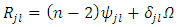 | (17) |
 | (18) |
where we introduced the identities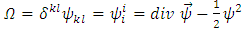 | (19) |
 | (20) |
 | (21) |
 | (22) |
Further, we try to find the physical significance of this Weyl vector field. Substituting the above identities into gravitational field equations (10), the Einstein tensor becomes | (23) |
Applying the partial derivative with respect to  , we get
  | (24) |
This Euclidean divergence of Einstein’s tensor is no longer identically zero. If we introduce the notation  | (25) |
after a rearrangement of terms, the Euclidean divergence of Einstein’s tensor can be written as follows  | (26) |
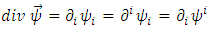
We can now observe that the expression  is the left – hand side of the differential equation which relates the magnetic vector potential to the electric current density, in stationary regim
 | (27) |
written in terms of components. Therefore, if we identify  | (28) |
where  is an arbitrary constant, the Weyl vector
  becomes proportional to the magnetic potential vector
  . With this identification, the expression (26) can be written again as follows
  | (29) |
where  are the components of the electric current density vector
  .
.
3. The Metric Tensor
According to (22) and (28), we have the relation | (30) |
Therefore, we can deduce  | (31) |
or | (32) |
Replacing this identity into (3), we obtain the metric tensor  | (33) |
4. Applications
In this section we calculate the magnetic vector potential and the well-known components of RC curvature tensor for different types of magnetic field.I) THE UNIFORM MAGNETIC FIELD In this application we calculate the vector potential and the components of RC curvature tensor, for a uniform magnetic field. We suppose that the magnetic induction is a vector parallel to the z axis, having a magnitude 
 | (34) |
For the magnetic vector potential, as in [4], we can use the formula 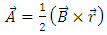 | (35) |
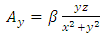
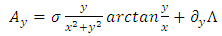
that yields the following expressions for its components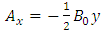 | (36) |
 | (37) |
Plugging these identities into (31), we get | (38) |
Thus  , and the metric tensor becomes
 | (39) |
Also, the RC curvature tensor vanishes | (40) |
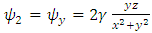
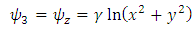
II) THE MAGNETIC FIELD OF A LONG STRAIGHT WIRE CARRYING CURRENT A straight wire by which the current I flows in the z direction produces, as in [5], the field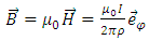 | (41) |
where 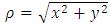 is the radial distance from the wire, and
 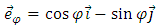 | (42) |
is the unit vector directed along the circumferential direction. The magnetic vector potential can be chosen as  | (43) |
where the two components have the expressions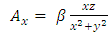 | (44) |
 | (45) |
and  is the constant
 | (46) |
Plugging these identities into (31), after integration, we get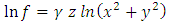 | (47) |
where  . From this we deduce
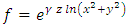 | (47a) |
We can now see that as  gets larger, so does
  . So this solution is not acceptable. Howbeit let us calculate further. If we substitute (47a) into (3), the metric tensor becomes
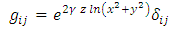 | (48) |
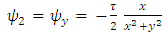
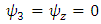
From (7) and (47), we find the identities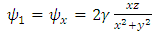 | (49) |
 | (50) |
 | (51) |
Substituting these identities into (15), we get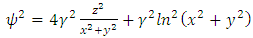 | (52) |
Substituting the identities (49) – (52) into (14), we find 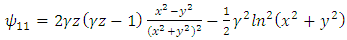 | (53) |
 | (54) |
 | (55) |
 | (56) |
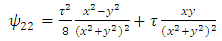
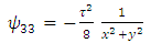
 | (57) |
 | (58) |
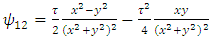
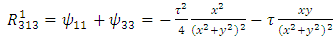
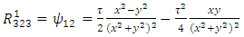
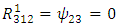
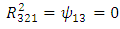
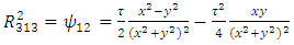
Plugging these identities into (13), we obtain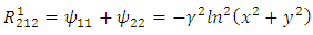 | (59) |
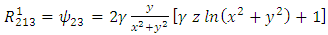 | (60) |
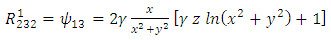 | (61) |
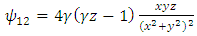
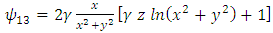
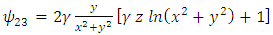
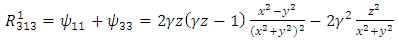 | (62) |
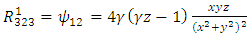 | (63) |
 | (64) |
 | (65) |
 | (66) |
 | (67) |
III) THE MAGNETIC FIELD GENERATED BY A CHARGE PARTICLE (ELECTRON) THAT PERFORMS A HELICAL MOTION For the study of this motion we assume that the electron is in rotation motion around the z axis, having the uniform angular velocity  | (68) |
In the same time, the electron is in translation motion along the z direction with the uniform velocity  | (69) |
The parametric equations of this helical curve are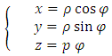 | (70) |
where  is the radial distance from the z axis, and
  is the helical parameter
 | (71) |
The equation (69) tells us that the electron produces a current  flowing in the z direction. For this component of current, we have to take into account the magnetic vector potential of a straight wire (43)
 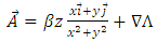 | (72) |
where, since the vector potential is not unique, we have added the gradient of an arbitrary gauge function. But, the equation (68) tells us that we also have a current  that flows in the sense of increasing
  . So, we have to take
  in the above expression of potential vector. Therefore, we obtain
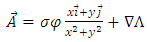 | (73) |
or, according to (70),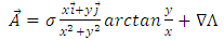 | (74) |
where  . The magnetic induction is obtained by taking the curl of this expression. Using the components
 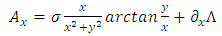 | (75) |
 | (76) |
 | (77) |
and the fact that  , we find
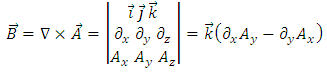 Therefore, the only non-zero component of
  is the z component
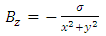 | (78) |
From the Stoke theorem, that relates the line integral of vector potential to the flux of magnetic induction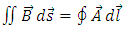 | (79) |
we can find the expression of gauge function  . Indeed, if we take a circular loop of radius
  centered along the z axis, the flux through the circular area is, as in [4]
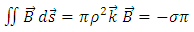 | (80) |
On the other hand, since the circuit element  is given by
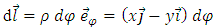 | (81) |
We find that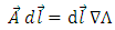 | (82) |
Therefore, the line integral of the potential vector may be expressed as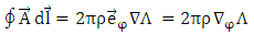 | (83) |
Now, from (80) and (83), we find the gradient of gauge function  as follows
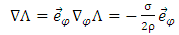 | (84) |
So, the gradient has a symmetric expression. If we use the spherical polar coordinates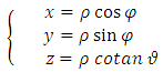 | (85) |
where  , the magnetic potential vector
  becomes
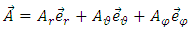 | (86) |
where the components are given by | (87) |
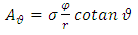 | (88) |
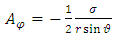 | (89) |
Finally, according to (84), we can write 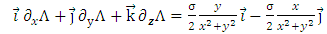 | (90) |
This equation gives us the expression of gauge function in Cartesian coordinates | (91) |
In spherical polar coordinates this function becomes | (92) |
So, it is a function of  only. If we substitute (86) into (31), after a simple integration, we obtain
 | (93) |
where  . This is a very similar situation to the previous application. As
  gets larger, so does
  . So, instead of trying to calculate again the components of RC curvature tensor, let us try the partial solution
  | (94) |
After a simple integration, we get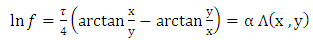 | (95) |
According to (7), this expression leads us to the following identities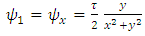 | (96) |
 | (97) |
 | (98) |
Substituting these identities into (15), we find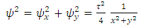 | (99) |
Substituting the identities (95) – (99) into (14), we obtain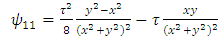 | (100) |
 | (101) |
 | (102) |
 | (103) |
 | (104) |
 | (105) |
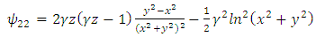
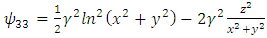
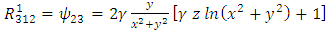
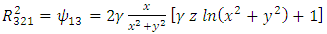
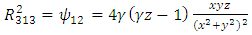
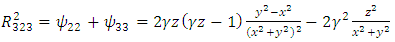
Therefore, the components of RC curvature tensor become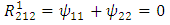 | (106) |
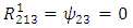 | (107) |
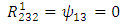 | (108) |
 | (109) |
 | (110) |
 | (111) |
 | (112) |
 | (113) |
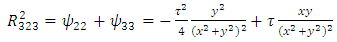 | (114) |
5. Conclusions
From the relation (33) of the metric tensor we can note that, if the magnetic vector potential is identically zero, then the metric tensor becomes
  , the curvature tensor components
  become identically zero, and the space becomes Euclidean. Thus, if there is no a magnetic field, then there is neither the curvature of space, nor gravity. Also, from the first application, we conclude that an uniform magnetic field does not produce a curvature of space, so does not produce gravitational field. From the next application, we can see that a variable magnetic field produces a curvature of space. But, from the identities (59) – (67), we can note that as
  approaches infinity, the curvature tensor, especially the
  component, approaches infinity. This result is not in agreement to the given physical situation. From (41), we observe that when
  gets to infinity, the intensity of magnetic field gets to zero. If a variable magnetic field produces a curvature of space, then the components of RC curvature tensor should approach zero when the intensity of magnetic field,
  , approaches zero. But, in our case, these components become infinite in the source and also to infinity. From the third application, we can note how can be removed this contradiction. Instead of the whole expression (74) of the magnetic vector potential
  , we introduced in the formula (30) only the gradient of gauge function,
  . In this way, we obtained appropriate solutions to the physical situation, because when
  approaches infinity, all the components of RC curvature tensor approach zero. This result is in agreement to the given physical situation.
References
| [1] | Weyl and Schrödinger — Two Geometries, William O. Straub, Pasadena, California 91104, April 20, 2015. |
| [2] | GHEORGHE VRANCEANU - Differential Geometry Lessons - Bucharest Teaching and Pedagogical Publishing House, 1976 - 1977, Volume 1 – Volume 2. |
| [3] | Simple Derivation of the Weyl Conformal Tensor, William O. Straub, PhD, Pasadena, California, April 14, 2006. |
| [4] | Magnetostatics III, Lecture 25: Electromagnetic Theory, Professor D. K. Ghosh, Physics Department, I.I.T., Bombay. |
| [5] | ELECTRICITY AND MAGNETISM – EDWARD M. PURCELL – Gerhard Grade University Professor, Harvard University, BERKELEY PHYSICS COURSE – Volume 2. |

 Abstract
 Reference
 Full-Text PDF
 Full-text HTML