Vlad L. Negulescu
Correspondence to: Vlad L. Negulescu, .
| Email: |  |
Copyright © 2017 Scientific & Academic Publishing. All Rights Reserved.
This work is licensed under the Creative Commons Attribution International License (CC BY).
http://creativecommons.org/licenses/by/4.0/

Abstract
This paper analyses the addition of velocities, forces and powers acting on an ideal particle, and represents a continuation and extension of the H-number model presented in an earlier contribution [1]. A hypothetical model, using the fact that mass flow rate is a tangent function, will permit the computation of the Universe’s mass.
Keywords:
Vector Hyper-complex numbers, Basic unit multipliers, Velocity, Force, Power, Geometrized system units, Big bang
Cite this paper: Vlad L. Negulescu, Addition of Velocities, Forces and Powers using Vector H-number Representation, International Journal of Theoretical and Mathematical Physics, Vol. 7 No. 3, 2017, pp. 57-60. doi: 10.5923/j.ijtmp.20170703.03.
1. Introduction
The calculus with hyper-complex numbers, or H-numbers, and their applications in physics were extensively presented in a paper [1], published in 2015. To be able to understand the present article the reader should first read it, especially the third chapter.
2. The V-H Numbers
2.1. Extension to H-numbers with Vector Parts
According to the article [1], an ideal particle is characterized by four parameters: time (t), mass (z), momentum (y) and space (x). This particle represents a point in the H space and can be written as an H number: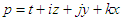 | (2.1) |
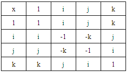
The four parameters of the particle are in expressed in meter, using the geometrized units System [2]. The symbols i, j and k are fundamental units of H-numbers. Table 1. Units’ Multiplication Table
 |
| |
|
If we consider that space and momentum are vectors, then the particle is represented by a Vector-Hyper-Complex number, or VH-number, which is formally written as: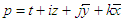 | (2.2) |
Where,  represents the scalar part of this number, and
  is the vector part. Its geometrical correspondence is a point in an eight-dimensional space.
2.2. Scalar and Vector Arguments
According to the paragraph 1.4 of the paper [1], an H-number can be exponentially represented by the following exponential expression: 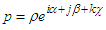 | (2.3) |
 is norm of
  is the imaginary argument,
  co-imaginary argument, and
  co-real argument. The notion of the unit multiplier is introduced in the paragraph 1.10 of the reference [1].The initial 3 basic unit multipliers will be now extended for vector-arguments:a. The rotor with imaginary argument is by definition a pure scalar
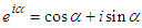 b. The rotor with co-imaginary argument contains a vector part:
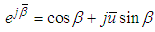 c. The pseudo-rotor with co-real argument contains a vector part, too:
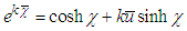 As you see we have introduced vector- arguments in the exponential expresion from b and c.
 where
where  and
and  are magnitudes and
  is a unit vector.The imaginary argument α is a scalar argument and the rotation
 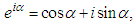 acts fully on any VH-number. The rules for unit multipliers with vector-arguments are postulated as it follows: The rotation with co-imaginary vector-argument and the pseudo-rotation with co-real vector-argument acts on the scalar part of any arbitrary VH-number. However they act only on the vector part which is parallel with their unit vectors. The perpendicular component remains unmodified.
3. Transformations for Particles with Constant Rest Mass
The present contribution analyses coordinate transformations, produced by multiplication with arbitrary unit multipliers, from the proper frame to a new frame. Further we will consider the particles with constant rest mass only, i.e.  where dz0 is the differential of the rest mass.
3.1. Multiplication by a Pseudo-rotor. Velocities Addition Formula
A particle in its proper frame is expressed by: | (3.1) |
where t0 and z0 are the proper time and respectively the proper mass. Now let us consider a differential mapping defined by the following expression: 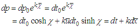 | (3.2) |
The velocity of the now moving particle is: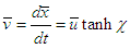 | (3.3) |
Let us analyze the case of two consecutive pseudo-rotations with arguments  and
and  . After the first pseudo-rotation we get:
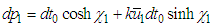 | (3.4) |
If the angle between the vector- arguments is Φ then we may write the components of dp1, which are parallel respectively perpendicular to  as it follows:
 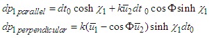 | (3.5) |
For simplicity reason the scalar part of dp1 was included in  The second pseudo-rotation acts only on the parallel component:
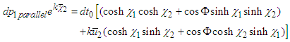 Finally it obtains
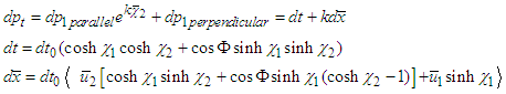 The resulting velocity is:
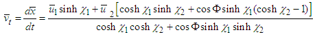 | (3.6) |
But the expressions of individual velocities can be written as: The final expression of the magnitude of the resulting velocity is:
 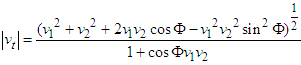 | (3.7) |
The above expression is symmetrical relative to v1 and v2. The absolute value of the velocity’s magnitude is less than or equal to 1 (light speed), as we already have expected.
3.2. Multiplication by a Co-imaginary Rotor. Forces Addition Formula
We start again with a particle at rest. The following mapping will be used: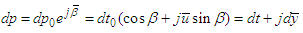 | (3.8) |
The force acting on the particle is: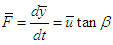 | (3.9) |
Now we will consider two successive rotations with co-imaginary arguments  and
and  . The mechanism of rotation acting on vector part follows the same rule as in the paragraph above.
 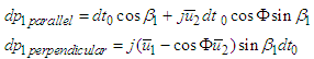 | (3.10) |
After the second rotation it obtains: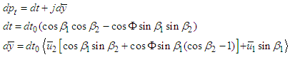 | (3.11) |
And thus we obtain the resulting force: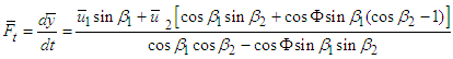 | (3.12) |
Writing the adding forces as: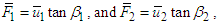 it obtains the magnitude of the resulting force:
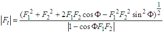 | (3.13) |
If the adding forces are parallel, then the resulting force is: 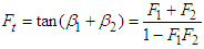 | (3.14) |
The conclusion of the analysis presented in this chapter is that forces are not adding linearly, as they use to do in classical mechanics and special relativity. However for practical cases this non-linearity is extremely small as we have mentioned in the previous paper [1] (see paragraph 2.10) published in 2015. The addition of two or more finite forces can result in an infinite one, because forces are tangent-functions. The reciprocal is also valid, i.e. an infinite force can be split in a number of finite individual forces.
3.3. Multiplication by an Imaginary Rotor. Powers Addition Formula
This kind of multiplication will keep the number representing the particle, in the complex plane, but its rest frame suffers a rotation with the angle α. The corresponding mapping is: | (3.15) |
The corresponding mass flow rate or power is: | (3.16) |
For P=0 we have the case of the constant mass  . For
. For  the mass is increasing, i.e. the system receives additional mass (energy) from the exterior. For
  the mass is decreasing, i.e. the system is losing mass (energy) to the environment. If we consider two successive rotations we came to the power addition formula:
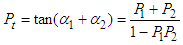 | (3.17) |
Because the power is also a tangent-function the addition of powers follows the same rules as the addition of forces. The addition of two or more finite powers can result in an infinite one, and an infinite power can be split in a number of finite individual powers.
3.4. Mass of the Universe
Let’s play a little around the power’s addition rule and tray to calculate the mass of the universe. We make the following assumptions:a. The big bang began 13.8 billons years ago, so the age of the universe is 4.32x10¹⁷ seconds [3]. b. The source was a singularity which contained an infinite power and consequently it has no proper time flow.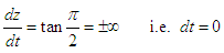 | (3.18) |
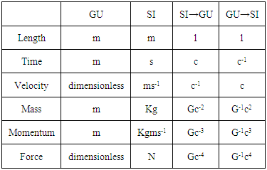
c. At the initial moment the singularity’s power made an abrupt transition from +∞ to -∞. Then this negative infinite power split in two finite powers P1=P2=-1, i.e. the total emerging power is 2. The power is expressed in geometrized units. d. Since then the mass flows uniformly in all directions. Let’s calculate the total emerging power (in SI units) using the following table (see [1] Table 2): The direct and reversed conversion international system of units (SI) to geometrized system of units (GU)Table 2
 |
| |
|
Using the values [4] of G and c in SI, the emerging power becomes: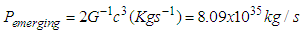 Age of the universe (tuniverse) is 4.32x10¹⁷ seconds.With all of these, the calculated mass of the universe is:
 It is obvious that this approach is only a hypothesis and the presented calculation a rough estimation. However, the above value belongs to the current estimated range which lies between 1053 and 1060 Kg, depending on different models and methods of calculation [5].
References
| [1] | Hyper-Complex Numbers in Physic, http://article.sapub.org/10.5923.j.ijtmp.20150502.03.html (accessed May 25, 2017). |
| [2] | Geometrized Units System, http://en.wikipedia.org/wiki/Geometrized_unit_system (accessed May 25, 2017). |
| [3] | The Universe by numbers, http://www.physicsoftheuniverse.com/numbers.html (accessed May 25, 2017). |
| [4] | Fundamental Physical Contacts, http://hyperphysics.phy-astr.gsu.edu/hbase/Tables/funcon.html (accessed May 25, 2017). |
| [5] | Mass of the Universe, http://hypertextbook.com/facts/2006/KristineMcPherson.shtml (accessed May 25, 2017). |

 Abstract
 Reference
 Full-Text PDF
 Full-text HTML