1. Introduction

In 1963 R. J. Glauber [1, 2] demonstrated that classical distribution functions for optical fields having no classical analogue can take on negative values. In general negative probability functions can express debt of probabilities when we use a classical tool to describe quantum dynamics. Traditional coherent-state description used by R. J. Glauber applied to photodetection related to normal ordering of field operators can be generalized to general operator orderings related to other detection possibilities, as introduced by K. E. Cahill and R. J. Glauber [3, 4] or more generally by G. S. Agarwal and E. Wolf [5-7], called s-ordering. Now many criteria exist how to recognize optical fields to be in nonclassical regimes [8, 9].

In last years we derived joint photon statistics including joint photon-number distributions and joint wave quasidistributions of the integrated intensities in classical as well as nonclassical regimes [10-12] (and references therein). These results can be applied, e.g. to Raman scattering [13], nonlinear optical couplers [14], and to entanglement of optical twin beams [15]. This theory is useful in analyzing experimental data [16-21]. Usually negative values of quasidistributions are related to nonclassical behavior of photon and wave statistics of the fields. Here we follow the way of arising singularities in the quasidistributions of the down-conversion optical process, also from the point of view of testing functions in the theory of generalized functions, in relation to nonclassical photon and wave statistics and illustrate procedures of regularization of singular quasidistributions. Such regularization procedures are able to eliminate singularities in the quasidistributions and can provide regularized quasidistributions reflecting nonclassical behavior of quantum systems by their negative values, which provides measurable quantities, in particular in terms of Laguerre polynomials. The results obtained can be applied to other nonlinear optical processes, such as Raman scattering, provided that classical strong coherent pumping fields are adopted.

2. Generating Function and Quasidistribution

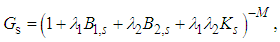
The generating function for the spontaneous optical down-conversion classically coherently pumped, determining measurable quantities, such as photocount distribution, its moments and wave distributions of integrated intensities, can be derived from the normal quantum characteristic function [22]

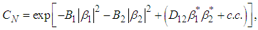(1)

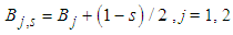
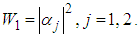
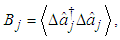where c.c. means the complex conjugation, β₁ and β₂ are parameters of the characteristic function, j = 1, 2, are mode quantum noise coefficients and a quantum correlation coefficient 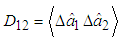in terms of annihilation operators and creation operators The normal generating function of the parameters and is then obtained as [22]

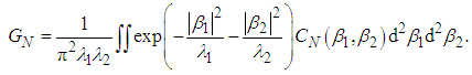(2)

Taking into account the s-operator ordering, we obtain for the generating function of the process

(3)

s is the ordering parameter (s = 1, 0, –1 for normal, symmetric and antinormal operator ordering) and the s-ordered quantum noise coefficients are defined as in terms of normal noise coefficients as follows from the theory of s-operator ordering [3-7], involving a filter function 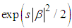in the quantum characteristic function of a parameter β; then 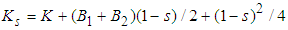. The parameter M represents the number of equally behaved modes (temporal, spatial and polarization in the spirit of Mandel-Rice formula) [10]; the quality of the process is characterized by the determinant involved in the Fourier transformation providing the Glauber-Sudarshan quasidistribution, whereas K_s is related in the same way for obtaining a quasidistribution related to s-ordering. The quantum (nonclassical) region is then defined by K_s < 0, whereas the classical one by K_s > 0 with the classical-quantum border K_s = 0 respecting the s-ordering.

For photodetection of optical fields we use the integrated intensity as a basic physical quantity defined as where t is initial time of a measurement, T is detection time and I is intensity of the measured field. If the detection space is equal to quantization space of the detected field, then where is a mode index describing temporal, spatial and polarization properties of the field and is a complex mode field amplitude. The joint quasidistribution of integrated intensities W₁ and W₂ related to s-ordering of field operators is then obtained by the inverse Fourier transformation from (3) as follows

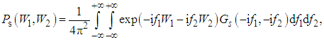(4)

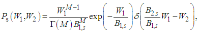
This double Fourier integral strongly depends on the sign of the determinant K_s. For K_s > 0 we can apply the Cauchy integral two times leading to the regular and nonnegative I_M–1-distribution [10-12] describing the classical behavior of the system as follows

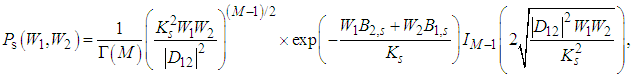(5)

where I_M–1 is modified Bessel function. For K_s = 0 the above distribution will be proportional to the Dirac δ-function [10] saying that the joint distribution is diagonal (as given in (8)).

For K_s < 0 we can use that the joint distribution is a generalized function and that the poles of the integrand in (4) are in the upper half-plane while the exponential function is analytic in the lower half-plane. Writing the denominator in (3) and (4) with the help of the following identity

(6)

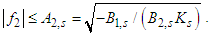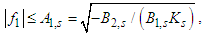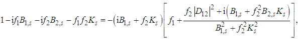
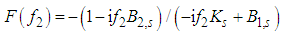
we see that we can calculate the Cauchy integral after f₁ in (4) in the lower complex half-plane if , which means that the Fourier variable f₂ is filtered and it holds that For frequencies outside this interval the pole is in the upper half-plane and the integral is zero. Changing the order of integrations, we change the indices 1 and 2 and we have and therefore is a band-limited function for any s. Performing the Cauchy integral after one Fourier variable, the integral after the other Fourier variable is band-limited and since K_s < 0, the poles in this integral lie in the upper-half plane and give no contribution [11, 12]. The resulting expression (see expressions (15) or (17)) is then symmetrized by multiplying the two results and taking the square root. In this way we have a regularized quasidistribution exhibiting nonclassical behavior by means of its negative values [10-13]. We traditionally use the joint regularized quasidistributions exhibiting negative values as reflecting nonclassicality [10-14]. In [23] the authors have used this principle in order to regularize the Glauber-Sudarshan quasidistribution constructing a filter function. In our case the regularization is performed naturally when considering the partially integrated joint quasidistribution for integration in the complex plane, thus smoothing singularities in the quasidistribution [11, 12]. Thus performing the integration along f₁ we obtain the following integral along f₂.

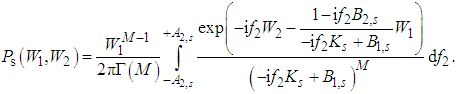(7)

At the quantum-classical border where K_s = 0 we obtain the δ-function diagonal distribution as mentioned above

(8)

with the corresponding threshold value of the ordering parameter

(9)

The system behaves classically if and in a quantum way if because K_s ≥ 0 and K_s < 0 in these cases, respectively.

3. Arising Generalized Function

In the following we will decompose the expression in the exponential function in (7) into the Taylor series and we will follow a way of arising singularities provided that the nonclassical regime with K_s < 0 occurs giving the pole in the upper half-complex plane, while the integral (7) is analytic in the lower half of the complex plane. Denoting in the exponential function in (7), we obtain for derivatives

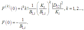(10)

From here we see that for k odd, are imaginary and for k even it holds for the coefficients of the Taylor decomposition that … are positive and 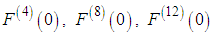… are negative if K_s < 0. This we use to calculate the corresponding integrals in the complex plane under the assumption that K_s < 0.

First include the terms up to the first power in f₂, which is equivalent to put K_s = 0 in all the terms starting with the terms containing giving the zero for the corresponding decomposition coefficients. In this case we can use the residuum theorem obtaining (the exponential function is now analytic in the upper half-plane)

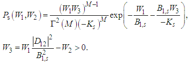(11)

In the opposite case the integral is zero because the exponential function is now analytic in the lower half-plane, however using (11) formally, we see that in this case the exponential function will be divergent and the power function will change the sign with M, which indicates nonclassical behavior in this case (which we will illustrate better by a regularization procedure in the following [11, 12]). The distribution (11) is regular and nonnegative and nonclassical behavior related to filtering of frequencies is lost here during the integration in the upper half of the complex plane along the infinite radius. The distribution (11) also represents a kind of smoothing of the diagonal distribution (8) compared to smoothing in terms of sinc-functions [10-12]. The distribution (11) is simplified if we put instead of close to the quantum-classical border, creating the symmetry of quantities and , giving

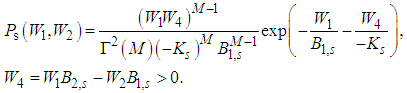(12)

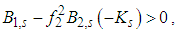
We can now consider integrals involving the Taylor series in the exponential function with the coefficients (10) provided that K_s < 0. We will successively consider approximate integrals with a finite number of the Taylor terms in the exponential taking into account that the last highest term is dominant. The integral (7) is zero because the pole lies in the upper half-plane for However, the integrals over give one because (7) is a distribution. Therefore its values at the zero are singular and we must have quasidistribution. Its behavior close to zero is like its asymptotic behavior in f₂, thus seeing that (7) exponentially diverges in in this case (in the classical case when K_s > 0 it goes to zero). We can use the path integrals along the lines given in Fig. 1 to illustrate their divergent behavior in nonclassical regimes. Denoting x = Re(f₂), y = Im(f₂), we have

(13)

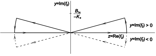Figure 1. Paths of integration in the complex f2-plane for Ks < 0; the full lines are for y = Im(f2) > 0 and dashed lines for y = Im(f2) < 0

Considering successively the integrals with k = 2, 3, 4, … we first conclude that all integrals with k odd are zero. Considering terms with we obtain that for the integrals about the segments vanish at infinity and because the pole is out the area of integration, the integral is zero with respect to the Cauchy theorem. If y > 0 we integrate along the full lines corresponding to if y < 0 we integrate along the dashed lines and the real axis corresponding to the dependence We can go with y to zero because the integral from to equals the complex conjugated integral from to and because the integral is real the result equals two times integral (7) and it is therefore zero. In these considerations the integral in (7) is taken from to because this integral is zero for filtered frequencies. If k is even and k = 4, 8, 12, …, we calculate the similar integrals along the path composed of full lines in Fig. 1 and the integrals are again zero along the segments at infinity provided that and we can go to zero with y again. For sufficiently small Im(f₂) ≠ 0, the modulus of the frequency is filtered. In general the non-zero imaginary part increases or decreases the maximum frequency of filtering in dependence on its sign. If k = 2, 6, 10, …, the corresponding integrals are divergent and they form the generalized function of the quasidistribution for K_s < 0. In fact the integrals with k odd include oscillating contributions of odd-order terms and we can only consider the integrals with the next even k.

In [23] singularities of the quasidistributions can also be considered from the point of view of testing functions in the theory of generalized functions [24]. In this context we see from (7) considering f₂ tending to that the testing functions must decrease more sharply than and thus they are members of the space Z of testing functions of the generalized functions in the space Z' [24], including the Glauber-Sudarshan quasidistributions [25]. Regularization procedures have long tradition [26, 27] and nonclassical filters can be used for them [28]. In the following we suggest particular regularization based on analytical properties of the generating function in the nonclassical region. It may be mentioned that conditions for testing functions obtained in [29] involve the decomposition of the exponential function contained in the photodetection equation to the power series, which provides rather formal mathematical conditions on the coefficients of the testing functions, whereas the explicit inclusion of the exponential function provides clear physical restrictions. Also series of derivatives of the δ-function are not suitable for physical reconstructions of quasidistributions, which can be realized effectively in terms of the Laguerre polynomials [22].

4. Regularization

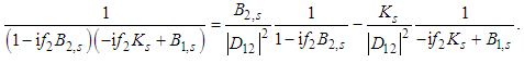
Thus for K_s < 0 we can regularize the integral in (7) integrating over W₂ (the integral along f₂ is to be regularized, the integral over f₁ was regular provided that the frequencies f₂ are filtered). In this way the factor –if₂ is added to the denominator in (7) (the pole if₂ = 0 just makes the regularization, in fact we have the Rayleigh (gamma) distribution in W₁). Now we can use the following identity

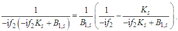(14)

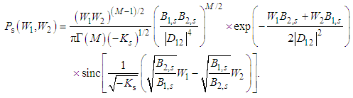
The second integral taken from to as a consequence of frequency filtering is zero because the pole lies in the upper half-plane and performing the derivative with respect to W₂ we have the same integral as in (7) with the denominator decreased by one, i.e. one factor is replaced by Successively we replace all these factors by including the denominator in the exponential function decomposing it in the series. If K_s > 0 leading to (5) the order of integration does not matter because both the variables f₁, f₂ are equivalent. However, in the nonclassical region where K_s < 0 the frequency filtering of one variable is necessary for performing the integration along the other variable and thus these variables are asymmetric now. Therefore we must perform the same calculation in the opposite order of variables changing the numbers 1 and 2 and taking the square root from the product of results and we then arrive at the final symmetrized regularized quasidistribution

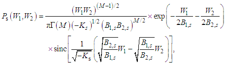(15)

where sinc(x) = sin(x)/x. When performing sampling of this quasidistribution [30] we make it first in W₂ following the order of integration (f₁, f₂) so that the frequency f₂ is filtered and then changing the order of integrations we make sampling in W₁, arriving at the same symmetric sampling formula; then the geometric average provides the final sampling with the symmetrized weighting function.

In principle we can also formally perform such a regularization over W₁ in (7) integrating per partes and using the identity

(16)

In the same way as above we obtain

(17)

This is a formal illustration because there is no need to regularize the Cauchy integral performed in f₁. Both the procedures are clearly the same at the quantum-classical border if we put B_1,sB_2,s instead of

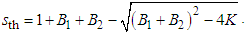
Thus we see that for K_s < 0 the wave statistics are characterized by the sinc-distribution taking on negative values with the maximum quantum effect for K = –B_j, where the joint photon-number distribution is diagonal, pointing out the two-photon quantum process [10]. The increasing K to 0 corresponding to the quantum-classical border finally gives the deterministic classical diagonal joint wave distribution with successively smoothing out the diagonal number distribution (the compound Mandel-Rice distribution [16, 17]), going finally to the isotropic joint distribution as the product of two Mandel-Rice distributions with no mutual correlations K = B₁B₂ > 0. The corresponding wave distribution is the I_M-distribution (5) with the product of two Rayleigh (gamma) distributions in the limit.

Even if we have considered the spontaneous process, the above conclusions are also valid for the stimulated process including a modulation factor involving I_M–1-function at the sinc-function in (15), under certain restrictions [31]. The above results are valid for all nonlinear processes, e.g. for Raman scattering, under the assumptions that their quantum statistics are described by Gaussian quantum statistics. This usually physically means that the nonlinear optical processes are pumped by strong classical coherent optical fields. Illustrations can be found in application to nonlinear optical couplers [14].

5. Conclusions

In this paper we have followed the way of arising singularities in the quasidistribution as reflecting nonclassical behavior of nonlinear optical parametric processes. Further we have developed regularization procedures providing regularized quasidistributions describing nonclassical behavior of quantum optical systems by their negative values. From them measurable quantities can be obtained permitting to follow evolution of quantum systems in their nonclassical regimes, which are available from quantum optical measurements. Although we have discussed spontaneous optical parametric processes, conclusions obtained are valid also for stimulated processes and for other nonlinear optical processes described by Gaussian nonclassical statistics, such as Raman scattering with classical coherent pumping. Here filtering of Fourier frequencies in nonclassical regions plays important role showing that the nonclassical quasidistributions are band-limited functions. All formulations are quite general involving s-ordering of field operators suitable for any kind of detection of the optical field including photodetection when normal ordering is appropriate.

ACKNOWLEDGEMENTS

The authors thank the support from the RCPTM project LO1305 of the Ministry of Education, Youth and Sports of the Czech Republic.