Bratianu Daniel
Str. Teiului Nr. 16, Ploiesti, Romania
Correspondence to: Bratianu Daniel, Str. Teiului Nr. 16, Ploiesti, Romania.
| Email: |  |
Copyright © 2016 Scientific & Academic Publishing. All Rights Reserved.
This work is licensed under the Creative Commons Attribution International License (CC BY).
http://creativecommons.org/licenses/by/4.0/

Abstract
Is already known that a non-inertial reference frame is equivalent to a certain gravitational field. In this paper, a non-uniformly accelerated linear motion of the reference frame is analyzed. We will try to prove that this motion generates a non-uniform and variable gravitational field, described by a Finsler metric. The attaching to the non-inertial reference frame of an electric charge, leads to changes in the structure of this gravitational field. The changes are produced by the EM radiation emitted, and can be easily recognized in the mathematical expression of the metric of space-time. The motion of the electric charge is analyzed also from a quantum perspective. The connection of the Schrodinger equation with the metric of space-time can be realized by means of a function of coordinates, which defines some Lorentz non-linear transformations. At the basis of these theoretical approaches is lay a variational principle in which the velocity of the particle is considered as a function of coordinates.
Keywords:
Damped quantum oscillator, Lorentz non-linear transformations, a different type of variational principle, Finsler space
Cite this paper: Bratianu Daniel, The Electromagnetic Radiation and Gravity, International Journal of Theoretical and Mathematical Physics, Vol. 6 No. 3, 2016, pp. 93-98. doi: 10.5923/j.ijtmp.20160603.01.
1. Introduction
Let us consider that we have a positive charge  located in the center of a inertial reference frame
  and a negative charge
  located in the center of a non-inertial reference frame
  Then, let us imagine that the non-inertial reference frame is moving with the acceleration
  in the (x) direction with respect to the inertial reference frame. Also, let us assume that the accelerated charge is moving such that the bilinear form
  | (1.1) |
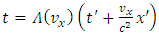
is an invariant with respect to the following non-linear transformations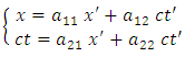 | (1.2) |
where,  So, we try to find the functions
  such that
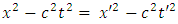 | (1.3) |
First we replace the coefficients  as follows
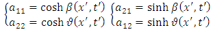 | (1.4) |
Then, substituting the transformations (1.2) into equation (1.3), we get | (1.5) |
So, we must have  and the transformations (1.2) become
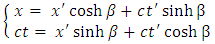 | (1.6) |
Also, we can admit the following inverse transformations 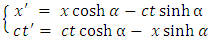 | (1.7) |
where  Differentiating now the direct transformations (1.6), we obtain
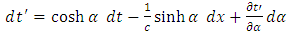
 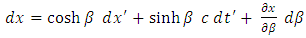 | (1.8) |
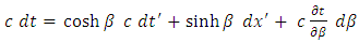 | (1.9) |
Differentiating also the inverse transformations (1.7), we obtain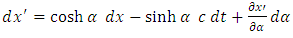 | (1.10) |
 | (1.11) |
In order to find the physical semnification of the function , we observe that, for the origin
  of the non-inertial reference frame, the equation (1.10) becomes
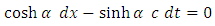 | (1.12) |
From this, we can deduce the derivative of the position  with respect to time
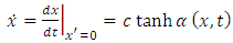 | (1.13) |
which signifies the velocity of non-inertial reference frame with respect to the inertial reference frame. Also, in order to find the physical semnification of the function  we observe that, for the origin
  of the inertial reference frame, the equation (1.8) becomes
 | (1.14) |
From this, we can deduce also the derivative of the position  with respect to time
 | (1.15) |
which signifies the velocity of the inertial reference frame with respect to the non-inertial reference frame. But, according to the motion relativity principle, we must have  | (1.16) |
Therefore, we can admit the following identity | (1.17) |
2. The Wave Function
Further on, we can associate a de Broglie wave with the accelerated charge. The wave must be stationary with respect to the non-inertial frame. Therefore, we can introduce the following wave function for the accelerated charge | (2.1) |
where  is given by the equation (1.7). Thus, we can rewrite this function with respect to the inertial reference frame as follows
 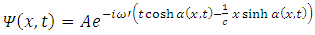 | (2.2) |
Taking the partial time derivative of this function, we get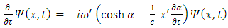 | (2.3) |
Now, we can introduce by definition the Hamiltonian operator 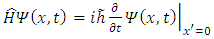 | (2.4) |
According to the equation (2.3), for the point  we get
 | (2.5) |
Therefore, we can deduce from here the following Hamiltonian function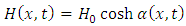 | (2.6) |
where  is the rest energy of the accelerated charge
 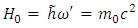 | (2.7) |
and  is the charge rest mass. Taking now the partial
  derivative of the function
  we get
 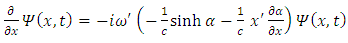 | (2.8) |
Further on, we can introduce by definition the linear momentum 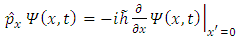 | (2.9) |
So, according to the equation (2.8), for the point  we can write
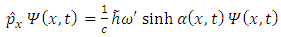 | (2.10) |
Thus, we obtain the following expression for the linear momentum of the accelerated charge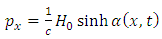 | (2.11) |
Substituting now the equation (1.13) into the equation (2.6), we get the well known formula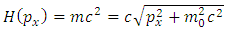 | (2.12) |
where  is the charge moving mass
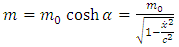 | (2.13) |
Also, substituting the equation (1.13) into the equation (2.11), we get the well known formula | (2.14) |
3. The Hamilton’s Equations
According to the principles of analytical mechanics, we can introduce now the Lagrange function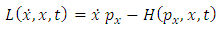 | (3.1) |
and the linear momentum  as the derivative of lagrange function with respect to
 | (3.2) |
where, according to the equation (1.13), we can consider | (3.3) |
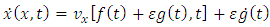
Let us consider also the action functional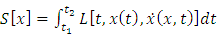 | (3.4) |
where  are constants. We assume that the action
  attains a local minimum at
  and
and  is an arbitrary function that has at least one derivative and vanishes at the endpoints
  So, for any number
  close to zero, we can write
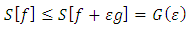 | (3.5) |
Thus, if the functional  has a minimum for
  the function
  has a minimum at
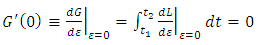 | (3.6) |
where, according to the equation (3.3),  and
and  are functions of
  of the form
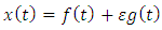 | (3.7) |
 | (3.8) |
Taking the total derivative of 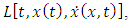 we get
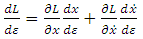 | (3.9) |
But, according to the equations (3.7) and (3.8), we have | (3.10) |
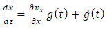 | (3.11) |
Therefore, we get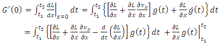 | (3.12) |
According to the fundamental lemma of calculus of variations, we get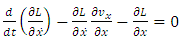 | (3.13) |
In consequence, we can introduce now the Hamiltonian function as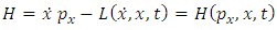 | (3.14) |
Differentiating now this function, according to the equation (3.13), we get the following equation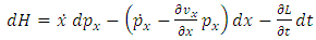 | (3.15) |
Comparing this expression with the mathematical expression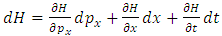 | (3.16) |
We get the following Hamilton equations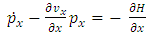 | (3.17) |
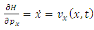 | (3.18) |
4. The Schrodinger Equation
Further on, we consider a function  which describes a physical quantity of the accelerated charge. Taking the total time derivative of the function
  we obtain
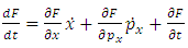 | (4.1) |
According to the equations (3.17) and (3.18), we can rewrite this formula as follows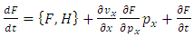 | (4.2) |
where  is the classical Poisson bracket
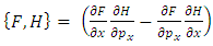 | (4.3) |
Let us write the equation (4.2) under the following form 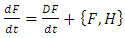 | (4.4) |
where  is an operator whose expression is given by
 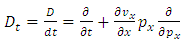 | (4.5) |
Taking into consideration the analogy between quantum mechanics and analytical mechanics, we can introduce an operator  corresponding to the physical quantity F. According to the equation (4.4), the corresponding equation for this operator must be
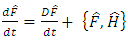 | (4.6) |
where  is the quantum Poisson bracket
 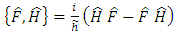 | (4.7) |
According to the equation (4.6), we can define the time derivative of the expectation value of the observable  as follows
  | (4.8) |
where  is the mean value (expectation value) of the observable
  Also, the law that describes the time evolution of a particle must be of the form
 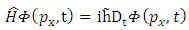 | (4.9) |
In this equation,  is the wave function of a quantum system, in the
  representation. According to this representation, the operators
  and
and  are given by the expressions
 | (4.10) |
Therefore, in the expression (4.5), we can make the replacing | (4.11) |
which leads us to the following expression of the operator  in the
  representation
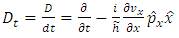 | (4.12) |
But we seek the Schrodinger equation (4.9) in the  representation. For this, we must introduce the operators
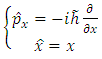 | (4.13) |
and the canonical commutation relation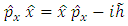 | (4.14) |
According to this relation, in the expression (4.12) we can make the replacing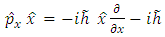 | (4.15) |
which leads us to the following expression of the operator  in the
  representation
 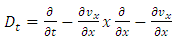 | (4.16) |
Therefore, we can write now the following Schrodinger equation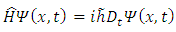 | (4.17) |
where the new Hamiltonian operator for the accelerated charge is given by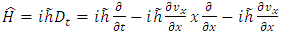 | (4.18) |
The additional term is of complex nature and its real part signify the potential energy of the field of force in which the particle is moving.
5. The Damped Oscillator
Let us consider that the accelerated charge  is bound to the fixed charge
  by an elastic force of the form
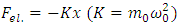 | (5.1) |
Taking the total time derivative of the equation (2.6), we can introduce, according to the special relativity theory, the following equation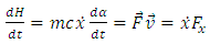 | (5.2) |
where  is the resultant force which acts on the accelerating charge
 | (5.3) |
This force must be the sum between the elastic force and the radiative reaction force | (5.4) |
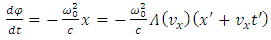
Therefore, for non-relativistic velocities, we get the equation of motion  | (5.5) |
We know that this equation is applicable only to the extent that the radiative reaction force is small compared with the elastic force This condition leads us to the following equation of motion
 | (5.6) |
where  | (5.7) |
Thus, the approximate solution of the equation (5.6) can be written as | (5.8) |
where  is the angular frequency of the damped oscillator
 | (5.9) |
Also, from the equation (5.2), for non-relativistic velocities, we can now deduce a new differential equation | (5.10) |
The integration of this equation leads us to the solution | (5.11) |
where  is given by the expression
 | (5.12) |
But, according to the equation (1.13), we must have the condition | (5.13) |
Taking the total time derivative of this equation, we get Now, we can replace
 Therefore, we get the equation
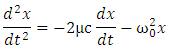 which is the same equation (5.6). Substituting this result into the equation (5.10), we can write the approximate equation
  | (5.14) |
The solution of this equation is given by the expression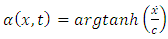 | (5.15) |
which results from the equation (1.13). Taking now the total time derivative of the displacement (5.8), we get | (5.16) |
This expression can be written as a function of the displacement function  under the following form
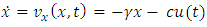 | (5.17) |
where the function  is given by the expression
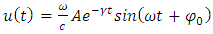 | (5.18) |
In this way, the velocity becomes a function of the coordinate  , because here the displacement
  is considered as a variable which no longer depends on time. Consequently, we may admit for
  a solution of the form
 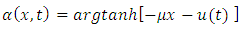 | (5.19) |
6. The Damped Quantum Oscillator
Substituting now the solution (5.17) into the equation (4.18), we get, for non-relativistic velocities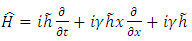 | (6.1) |
For the Hamiltonian operator of the oscillator, we take the expression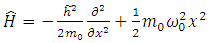 | (6.2) |
Admitting for the wave function a solution of the form 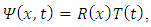 after the separation of variables, we get the following two equations
 | (6.3) |
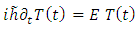 | (6.4) |
where the constant  is the separation constant, and signifies the total energy of the quantum oscillator. Thus, after a rearrangement of the terms, the first equation can be rewritten as follows
 | (6.5) |
Further on, we can introduce a dimensionless variable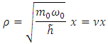 such that the equation becomes
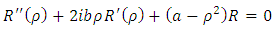 | (6.6) |
in which we have introduced the notations | (6.7) |
 | (6.8) |
 | (6.9) |
Now, we can take for  a solution of the form
 | (6.10) |
which generates the differential equation for the unknown function 
 | (6.11) |
The constant  can be determined from the equation
 | (6.12) |
In order to get a finite solution for the function  we choose the root
 | (6.13) |
where we have introduced the notation | (6.14) |
Therefore, the equation (6.11) becomes | (6.15) |
We can introduce now a power series expansion as solution | (6.16) |
Substituting this expansion into the differential equation (6.15), we get | (6.17) |
which leads us to the recursion relation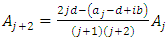 | (6.18) |
Because the series must be finite, there exists some  such that when
  the numerator will be zero. Therefore, we get
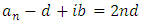 | (6.19) |
Substituting here the formula (6.8), we obtain the following complex expression for the total energy of the quantum oscillator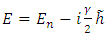 | (6.20) |
where  are the quantized energies of the quantum oscillator
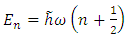 | (6.21) |
Substituting now the constant  into the expression (6.10), we get
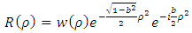 | (6.22) |
Also, substituting the equation (6.19) into the equation (6.15), we get for the unknown function  the equation
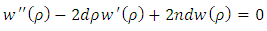 | (6.23) |
If we introduce now a new dimensionless variable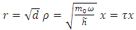 | (6.24) |
the equation (6.23) becomes 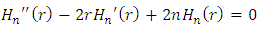 | (6.25) |
where  are the Hermite polynomials. So,
 and the solution
  can be written as
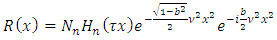 | (6.26) |
where  are the multiplication factors, whose expression can be determined by the normalization condition of the wave function.For the second equation (6.4), we have the solution
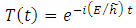 | (6.27) |
Substituting here the solution (6.20), we get the expression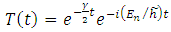 | (6.28) |
which describe the time evolution of the wave function for the accelerated charge.
7. The Metric of Space-Time
Let us write now the “distance” between two infinitesimally close events, into the inertial reference frame 
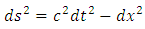 | (7.1) |
Substituting here the equations (1.8) and (1.9), we get | (7.2) |
where the components of the metric tensor are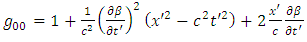 | (7.3) |
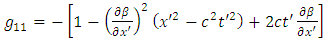 | (7.4) |
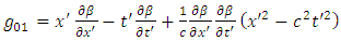 | (7.5) |
But, according to the equations (1.17) and (5.11), we have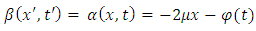 | (7.6) |
Then, according to the transformations (1.6), we can impose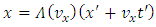 | (7.7) |
 | (7.8) |
where 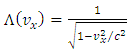 | (7.9) |
Substituting now these expressions into the equation (7.6), we get | (7.10) |
where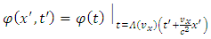 | (7.11) |
Taking now the partial  derivative of
  we obtain
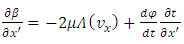 | (7.12) |
Also, taking the partial  derivative of
  we obtain
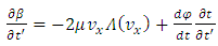 | (7.13) |
But, according to the transformations (7.7) and (7.8), we can write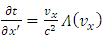 | (7.14) |
 | (7.15) |
 | (7.16) |
Substituting these expressions into the equations (7.12) and (7.13), we get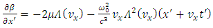 | (7.17) |
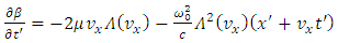 | (7.18) |
where the velocity  is given by the expression (5.17), which no longer can be written as a function of the coordinates
  So, in this particular case, the metric of space-time (7.2) becomes a Finsler metric, and the space becomes a Finsler space.
8. Conclusions
Intuitively, the non-uniformly accelerated linear motion of a oscillator must be equivalent to a uniform but variable gravitational field. However, the gravitational field described by the metric of space-time (7.2), is a non-uniform field. This is due to the particular mode of writing of the velocity of a particle as a function of the coordinates  and the function
  depending on the same coordinates, by means of the velocity. Also, from the equation (3.17), we can observe that the term
  corresponds at the half of the radiative reaction force
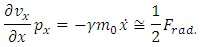 Therefore, the function
  which determines the Lorentz non-linear transformations, intervenes in the determination of the radiative reaction force of the EM field and, also, in the determination of the gravitational field which appears in the non-inertial reference frame. Indeed, if we impose now
  we get
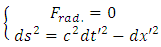 so, both, the radiative reaction force and the gravitational field, vanish. On the other hand, the radiative reaction force vanishes again when the oscillator is a neutral particle, but the gravitational field does not vanish, because
  is different from zero. This suggests that the EM energy carried by the EM radiation contributes to the energy of the gravitational field. Also we can conclude that the field which appears as an EM field into the inertial reference frame, appears as a gravitational field into the non-inertial reference frame.
References
| [1] | The Classical Theory of Fields, Third Revised English Edition, Course of Theoretical Physics, Volume 2, L. D. Landau and E. M. Lifshitz, Pergamon Press, 1971. |
| [2] | General Relativity and Cosmology, by Nicholas Ionescu-Pallas, Scientific and Encyclopedic Publishing house, Bucharest, Romania 1980. |
| [3] | From Albert Einstein to R. G. Beil, by Valentin Gartu, Fair Partners Publishing house, Bucharest, Romania 1999. |
| [4] | General Physics, by Traian Cretu, Technical Publishing house, Bucharest 1984. |
| [5] | The Meaning of Relativity, by Albert Einstein, Princeton University Press, Princeton, New Jersey 1955. |

 Abstract
 Reference
 Full-Text PDF
 Full-text HTML