1. Essentials: Testing for the Semi-Exactness and Non-Exactness of Equations and the Two Methods of Determining Integrating Factors. The Three Methods of Solution of Semi-exact Equations

Are integrating factors for semi-exact equations determinable in principle? Quotation: “There is no general method for finding an integrating factor, but a familiarity with differentiation formulas will sometimes help in determining them” [1]. We do not quite agree to the first part of this statement, and we are certainly not in the dark about the determination of integrating factors for the semi-exact equations. Actually the topic of integrating factors is still confused in the literature due to failure to recognize the connection between the integrating factors and integration by parts and the distinction between the separating and integrating factors. However, this ambiguity will be removed and a clearer and wider coverage of the topic of integrating factors will be attempted in this work.

A clear understanding of the topic of semi-exact equations and their integrating factors cannot be attained before acquiring the capability of recognizing and distinguishing the complexity of concepts underlying the said topic. Semi-exact equations can be classified as: two-variable, but hardly three-variable equations; two-term, three-term, and multi-term equations; equations with and without non-homogeneity terms; equations with singlet and non-singlet non-homogeneity terms, and ; equations with doublets having exact and semi-exact dependent and independent arms; equations with two or more semi-exact doublets requiring the same integrating factors; equations with one-variable and two-variable integrating factors; equations with first and second order doublets; equations with doublets having simple and composite arms. There are also: separating and integrating factors; separated, separable, and inseparable equations; separable semi-exact and separable non-exact equations; equations separable by separating factors and by substitution (change of variables); separable equations with simple and composite singlets; determining integrating factors by partial differentiation and by test-by-sight, … etc. We should be able to move with clear visibility through such multi-branched complexity of interrelated concepts. Insisting on full understanding, right from the outset, of each of these concepts individually within their wide range of interrelated complexity, at the expense of sacrificing the clarity of their interrelations, may not be the best method of dealing with the subject. It may be more beneficial to be satisfied in the beginning with partly understood multiplicity of concepts so as to concentrate on their interrelations, and then return to their full understanding thereafter. This is somewhat similar to indexing of articles in a spare parts store, or writing the page of “contents” in which the titles of the chapters of a book are gathered for general framing of the topic to be studied. This second approach is followed so as not to lose one’s way in a forest of concepts and ideas. In this work a mixture of the two approaches will be tried in [part A], and the full understanding of the topic will be attempted in [parts B and C].

1.1. The Separable Semi-exact, and Separable Non-exact Equations

In the relevant text-books the exactness and semi-exactness of equations and the two partial differentiation tests for establishing them (and determining the integrating factors in the case of semi-exactness), and finally the related examples and exercises and their solution by “ integration in total differentials” are dealt with in certain sections allocated to the topic in these text-books. It is important to note that outside these sections in these text-books themselves, it is almost a constant practice to overlook all that has been stated above about the exact and semi-exact equations and, instead, a strong tendency is often revealed to solve these equations by “separation of the variables” without realizing their being exact or semi-exact or recalling to apply the relevant tests for ascertaining the kind of the given equation. The “separable semi-exact equations” are, as their name implies, solvable by the two methods above, but it is more convenient to apply the third method of “integration by parts” which is much shorter and simpler. On the other hand the “separable non-exact equations” are, again as their name implies, not solvable by integration in total differentials, or integration by parts, but only by separation of the variables. Being the only applicable method in this case, the separation of the variables should unavoidably be applied and its comparative prolongation should, of course, be tolerated. It is also important to note that in exemplifying the separation method text-books ought not to select their examples from the separable semi-exact equations, and face the anecdotal situation of solving by a prolonged method (separation of the variables to be exemplified) when a much shorter method (integration by parts) is within reach. They ought to select their examples from the separable non-exact equations so as to leave no choice but applying the method to be exemplified.

1.2. The Two-term, Three-term, and Multi-term Semi-exact and Non-exact Equations

Distinction should be made between the two-term and three-term equations (not to be confused with the two-variable and three-variable equations).

(a) The two-term separable semi-exact equations and their three alternative rectifying factors: These equations, which are encountered occasionally, possess three alternative factors each of which alone can accomplish the integration of these equations. For instance, the equation has one separating factor , and two integrating factors: , and (since x and y can exchange freely their roles of being the dependent and independent variables in a two-term equation). It is to be recalled that the separating factors are used in the method of separation of the variables (simple, or composite singlets) followed by term-wise integration by the basic formulas, whereas the integrating factors are used in integrating doublets (and triplets) by parts (in addition to the term-wise integration of singlets in three-, and many-term equations). The same general solution of the given equation will be obtained by using any of the said three factors. On the other hand, a separable non-exact equation has a separating factor, but no integrating factor. Obviously the two kinds of factor and the three methods of solution represent distinct techniques in solving semi-exact equations.

(b) The three-term semi-exact equations and their three component rectifying factors: These equations are with one-variable, and two-variable integrating factors. The equations with one-variable factors are encountered more frequently than those with two-variable factors, and the two kinds of equation constitute the basic group of semi-exact equations. These equations are usually solved by separation of the variables by substitution, i.e., by solving the corresponding homogeneous equation for the complementary function, and applying variation of parameters for the particular integral (see Examples 1, 2, and 3). We shall, however, discard these comparatively prolonged techniques and apply the much shorter and simpler methods of test-by-sight (i.e., the three-rectification process for finding integrating factors), and of integration by parts for performing the solution. These equations consist basically of three constituents: the non-homogeneity term, and the two dependent and independent arms reciprocated in a doublet of terms. Each of the three constituents may require its own rectifying factor (r₁, r₂, r₃). These equations have only one integrating factor which is, generally speaking, the product of the three rectifying factors, that can be easily determined by sight. Equations for which any of the three rectifying factors is indeterminable are non-exact equations. This will be explained later in [part A-4-b].

(c) The multi-term equations with two or more semi-exact doublets requiring the same integrating factor: The semi-exact equations with four, five, six, and seven terms necessarily contain “two semi-exact doublets requiring the same integrating factor” otherwise they are non-exact. Note that a doublet is either simple (with two terms), or composite (with three terms), and furthermore these equations are either “with” or “without” a singlet non-homogeneity term. Accordingly, these semi-exact equations can be:

i- Four-term equations (with two simple doublets and no non-homogeneity term, see Exercise 7).

ii- Five-term equations (with two simple doublets and a non-homogeneity term, or with one simple and one composite doublets and no non-homogeneity term, see Example 4).

iii- Six-term equations (with two composite doublets and no non-homogeneity term, or with one simple and one composite doublets and a non-homogeneity term).

iv- Seven-term equations (with two composite doublets and a non-homogeneity term).

v- Linear n-th order equations with constant coefficients (can be rearranged as a sum of “n” semi-exact doublets requiring the same integrating factor- see Example 7).

Outside these combinations of terms there exist “multi-term non-exact equations”. Being “diversified by adding more terms”, these equations may have, due to their too many terms, “inconsistent rectifying factors” resulting in the non-exactness of these equations for which no integrating factors exist and to which integration by parts does not apply.

1.3. The Two Methods of Determining Integrating Factors. The Separating Factor for Composite Singlets

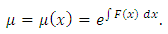
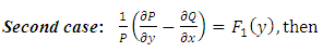
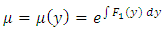
Integrating factors can be obtained by two distinct methods: (1) by the formula derivable by partial differentiation [for obtaining one-variable integrating factors, i.e., either , or , but not ], and also derivable by integration by parts as will be shown in [Example 5], and (2) by the newly introduced “three-rectification process” (performed by test-by-sight based on integration by parts). This latter method is used for obtaining both of the one-variable, and two-variable integrating factors. We also note that the separating factor of composite singlets, , obtainable in some obvious cases by sight and not by partial differentiation, is usually confused with the integrating factor (see the third quotation below). Distinction between the separating and integrating factors together with the two methods for finding integrating factors, will be discussed later.

1.4. The Three-, Two-, and One-variable Integrating Factors

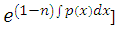
(a) Evading the three-variable semi-exact equations and the three-variable integrating factors: Whereas the three-variable exact equations are common in the literature, the three-variable semi-exact equations are hardly encountered. Suppose we took some arbitrary exact equations and divided them by some arbitrary one-, two-, and three-variable functions: , , and , then we would obtain a wide range of semi-exact equations for which the said functions would be integrating factors of all sorts. Except for some obvious cases most of the semi-exact equations obtained in such a crooked manner, especially the three-variable equations, would be too artificial and extremely difficult to identify by sight. It would hardly be possible to determine the integrating factors for such artificially constructed semi-exact equations to accomplish their integration. Because of this obvious difficulty the three-variable semi-exact equations are not encountered (unlike the case of exact equations), and consequently, the three- variable integrating factors, , are likewise unheard of. With the three-variable semi-exact equations excluded from usage, the term “two-variable semi-exact equations” will be abbreviated in this work from now on simply to “semi-exact equations”. There will be no further mentioning of this contraction which is to be understood impliedly where it arises.

(b) The semi-exact equations with two-variable integrating factors obtainable by the “three-rectification test by sight” and not by “partial differentiation”. Bernoulli’s equation can serve as a typical example of such equations. As mentioned earlier, the two-variable total integrating factor is the product of three component rectifying factors: [R(x,y) = r₁r₂r₃]. Factor r₁ is to rectify (i.e., prepare for integration) the non-singlet non-homogeneity term, q₁(x,y), by turning it into a singlet, q₂(x), individually integrable by the basic formulas. Only when the non-homogeneity term is in the form of the product can it be rectified by multiplying the equation by factor . If this condition is not satisfied the equation is non-exact. Factor r₂ is a constant to rectify (make exact) the already semi-exact dependent arm “solely created or altered” by the first rectifying factor as is evident in the five examples below. This arm can be rectified only by and not by since the latter would return the singlet back into a non-singlet and invalidate the “individual integrability of the non-homogeneity term”. An would make an equation non-exact. Finally factor is to rectify the semi-exact independent arm and consequently the doublet to be integrated by parts. It is important to keep in mind that this “three-rectification process for determining integrating factors” should be applied in the above-stated order (r₁,r₂,r₃) to avoid the possibility of a latter factor invalidating the rectification achieved by a former factor or factors. It is also important to recall that factor r₂ is determined after multiplying the equation by r₁, and factor r₃ after multiplying by r₂. It should also be noted that when x and y exchange their roles of being the dependent and independent variables then it is the factor f (x) that should be deleted from the non-homogeneity term by division and [v(x)→ v'(x)] becomes the dependent arm. Only by decomposing the given three-term equation mentally into its three basic constituents is it possible to establish by sight the semi-exactness (or, non-exactness) of the equation and determine, in the case of semi-exactness, the three component rectifying factors that constitute the total integrating factor of the equation. Equations to which the three-rectification process applies (i.e., in which all the three rectifying factors are determinable) are semi-exact equations. On the other hand, equations to which the said process is inapplicable (i.e., in which at least one of the three rectifying factors is indeterminable) are non-exact equations for which no integrating factors exist. That is simply the condition whose presence and absence determine the semi-exactness and non-exactness of a given three-term equation respectively. The multi-term equations with two semi-exact doublets are also included. If the two doublets require the same integrating factor the equation is semi-exact and if the required integrating factors are different the equation is non-exact. The said processes will become clearer when we revise the solutions of [Examples 1 and 4 of sec. B].

Below are five examples of semi-exact equations with two-variable integrating factors. In the first four examples the functions of the independent variable are in the general algebraic form, and , whereas those of the dependent variable are in specified functional forms: , These equations satisfy the above stated conditions for “semi-exactness with two-variable integrating factors”. The equations are two-variable, three-term, non-linear, first order equations. Their three basic constituents are rectifiable in the stated succession . Their non-homogeneity terms are non-singlets in the form of a product rectifiable by division. It is to be asserted that the semi-exact equations with non-singlet non-homogeneity terms, , possess two-variable integrating factors, , whereas equations with singlet non-homogeneity terms, , possess one-variable integrating factors, . After multiplying the equations by the resulting semi-exact dependent arms are rectifiable by constant multipliers . Their independent arms are rectified by . These equations are solved in three steps: rearranging the given equations such that the doublets are put on the left side and the non-homogeneity terms on the right side of the equations, multiplying by the integrating factors obtainable by sight in the sequence already mentioned, and integrating (by pair-wise and term-wise integrations) the resulting exact doublets and the singlet non-homogeneity terms respectively.

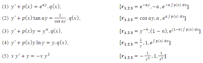To solve the fifth equation, as an example, by the three-rectification method we first note that the equation needs no rearrangement of its terms and factors. It is initially with an exact doublet , but this is needed after rectifying the non-homogeneity term by (which may cancel the exactness but retains the semi-exactness of both of the dependent and independent arms to be rectified by respectively). If the equation is divided by it becomes a Bernoulli’s equation with . The presence of means that the is the dependent arm and that the non-homogeneity term should be rectified to . We, therefore, multiply by and obtain . The remains exact in its new form in this example, i.e., . 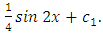As will be explained later, for the x-arm is . We thus obtain the exact equation . We then integrate (by multiplying the outer functions of the exact doublet) to get . The fifth equation is also solvable by the ready formula to be derived in [Example 1]. The usual (prolonged) solution is by separation of the variables by substitution. Furthermore, with its two-variable integrating factor being indeterminable by partial differentiation the equation cannot (and need not) be solved by the (prolonged) integration in total differentials (without the integrating factor having been obtained in advance). Note that most of the statement above is not a part of the written solution but an explanation of the methods applied and applicable to the given problem.

(c) The semi-exact equations with one-variable integrating factors obtainable by partial differentiation and by test-by-sight: This is the prevailing case of semi-exact equations and their integrating factors, i.e., most of the frequently encountered semi-exact equations belong to this category (see the first half of the table in [part A-6] below.

i. The first order equations with singlet non-homogeneity terms and exact dependent arms, and their integrating factor : The first order equations (linear and nonlinear, with constant and with variable coefficients) can be told by their forms, i.e., they are identifiable by test- by- sight. They constitute an important class of semi-exact equations with one-variable integrating factors . This is another way of saying that the singlet non-homogeneity term and the exact linear or nonlinear dependent arm of the doublet are already given in rectified forms and only the semi-exact independent arm requires the integrating factor to become rectified, i.e., an exact arm: , (note that the arrow extends from the exponential function to its derivative). The said integrating factor is already known, and derived by partial differentiation as in (ii) below, but in current use it is still far from being properly understood. We will, however, remove the ambiguity when we revise the solution of the first order equation 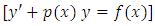in [Example 5], and derive this integrating factor by the much simpler method of integration by parts.

ii. The partial differentiation test for determining the integrating factors: or but not . Three quotations.

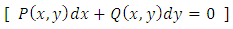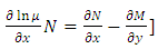
The first quotation: “If the left side of equation is not a total (exact) differential, then there exists a function (integrating factor) such that 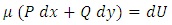. Whence it is found that the function satisfies the equation 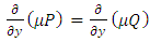. The integrating factor is readily found in two cases:

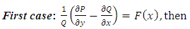
” [2,3]. The details of the derivation will be given in [Example 4].

The second quotation: “Of course it is not always so easy to find the integrating factor…, In the general case, integrating this partial differential equation is by no means an easier task than integrating the original equation… we can find the conditions for the existence of integrating factors of the form 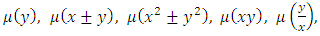and so forth” [4].

The third quotation: two solved examples:

First example: “Does the equation have an integrating factor of the form

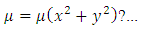
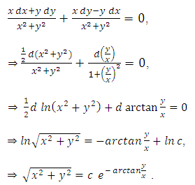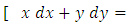
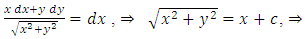
Second example: The equation has the obvious integrating factor . (We thus have): . (a family of parabolas)” [4]. The three quotations above will be analyzed below.

iii. Distinction between the integrating and separating factors in the above quotations.

[Note: Integrating factors are denoted by in this paper, but by in the quotations above. Also the functions denoted by P and Q in the first quotation are denoted by M and N in the second quotation (which is from a different reference). This formal note ought to be recalled to avoid possible confusion].

(a) The implication is obvious in the first quotation that after transforming a semi-exact equation by its integrating factor into an exact equation, the solution will be by integration in total differentials, and not by separation of the variables, or by integration by parts. As was asserted in our first paper, the method of integration in total differentials is no longer required, having become comparatively laborious and prolonged where a much shorter and simpler method is within our reach, namely, integration by parts. It is this short-cut in the solution what permits the distinction between the three methods of solution and between the two separating and integrating factors. Furthermore, the quotation, in effect, erroneously implies that integrating factors are not connected with integration by parts, since it is integration in total differentials and not integrations by parts that is applied, according to this quotation.

(b) As is explicit in the first and second quotations, the one-variable integrating factors, and , are derivable by the partial differentiation method (as will be detailed in Example 4), (and by the much simpler integration by parts, as will be shown in Example 5). The factor applies instead of to equations so presented that x and y exchange their roles of being the dependent and independent variables. It is also explicit in the second quotation that a general method for finding the two-variable integrating factors by derivation from first principles (i.e., by partial differentiation) does not exist (only the three-rectification test by sight is now available for obtaining these factors).

(c) The two-variable factors stated in the second quotation and applied to the two solved examples in the third quotation are not integrating, but separating factors. These factors transform the given equations into “separated equations with composite singlets”. Contrary to the assertion of the first quotation, “we saw no formulas for integration in total differentials applied to the solution of the two examples in the third quotation”. This observation obviously excludes integration in total differentials in favor of the method of separation of the variables (with the method of solution by integration by parts assumed not to have been recognized as yet). The two examples were actually solved by term-wise integration by the basic formulas, i.e., by “separation of the composite variables”, not by substitution, but by separating factors as we saw in the two-term equations. The quotation also implies that what it regards as integrating factors are associated this time with the method of separation of the variables (which actually employs separating factors or substitutions and not the integrating factors associated with integration by parts). The separating factors stated in the quotation are moreover not derived by a general method (i.e., by partial differentiation), but only guessed at in some obvious cases as already stated in the quotation itself. Of course, what matters in the first place is to solve the given equation by whatever method, but when more than one method become available then it also matters (in the second place) to specify which of the methods is the most convenient for application (which is in fact the subject-matter of our first and second papers).

iv. More notes about integrating factors:

In addition to the three notes about integrating factors inferred from the above quotations there are three other notes to be added.

(a) By using the formula the first part of the table compiled in [A-6] can be derived. However, obtaining integrating factors by written derivation using the said formula is hardly necessary in actual practice, nor is it necessary to consult the said table either. A moment of reflection about the semi-exact independent arm and how to turn it into the exact arm will suffice to determine the integrating factors by test-by-sight. That is actually how the table was compiled.

(b) We shall call the expression an “exact second order doublet” with the arms and . The “semi-exact second order doublet” possesses two integrating factors either of which can be used in the first integration and the other is neglected (cannot be used in the second integration) (see the second part of the table and Example 6).

(c) The n-th order linear equation with constant coefficients is an n-step semi-exact equation possessing n integrating factors that can be used for n successive integrations of the equation by parts. This will lead to the derivation of a readily applicable generalized formula for obtaining the general solution (complementary function CF + particular integral PI) of the given equation. (see Example 7).

1.5. The Non-exact Equations

Whereas the exact three-term equations can be diversified by adding more terms and making them with more than one non-homogeneity term, with more than one doublet, and/or with one or more triplets, such diversification of equations by adding more terms is generally not possible in the case of semi-exact equations (except for the equations with two or more semi-exact doublets requiring the same integrating factor). This impossibility arises from the fact that by adding more terms to an equation the rectifying factors would then be too many to match together, i.e., they would uncontrollably invalidate the rectifications achieved by the different factors and prevent the existence of a total integrating factor. The three-term equations become non-exact if their non-singlet non-homogeneity term is other than a product separable by division, or if one of the three y’s (in the non-homogeneity term and in the functions of the dependent arm) is the argument of other than a power function, or if the difference between the exponents of the y’s in the dependent arm is not “unity”in a first order doublet, and not “two” in a second order doublet. The presence of these characteristics in an equation and of the previous characteristics of “diversification of equations by adding more terms” is the cause of the non-exactness of this class of equations, and of the non-existence of integrating factors for them.

In answer to the question we started with, and excluding the three-variable semi-exact equations for the reasons already mentioned, it can be asserted that the one-variable and two-variable integrating factors for the semi-exact equations are determinable in principle. The semi-exact equations are amenable to the three-rectification process thanks to their possessing the characteristics (conditions) already mentioned. Equations lacking any of the said characteristics are non-exact equations which are insolvable by integration by parts. However, some non-exact equations are separable and, therefore, solvable by the separation method. The above multi-sided discussions of the topic of integrating factors will now be finalized with a table compiled for these factors in [part A-6] below before reworking the seven examples of [part B] by obtaining their integrating factors by sight and their solutions by integration by parts.

1.6. A Table of Integrating Factors Easily Identifiable by Sight for the Frequently Encountered Equations with Semi-exact First and Second Order Doublets

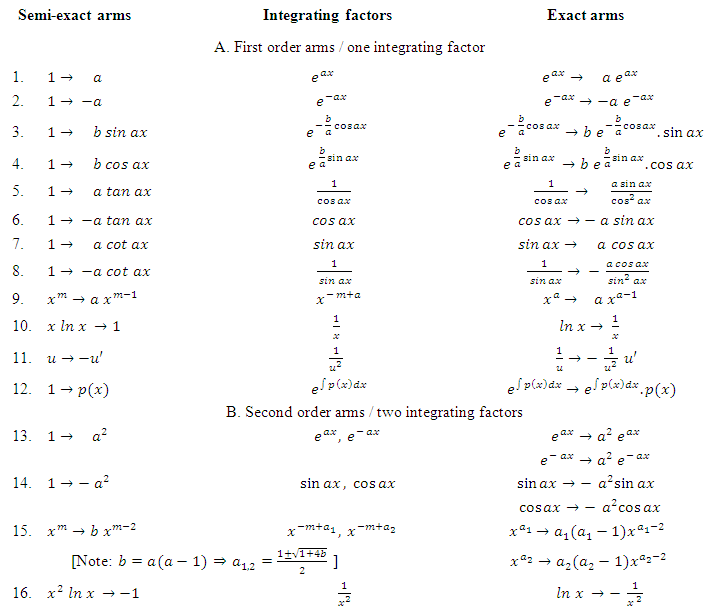Note: The first part of the table applies to the equations with first order doublets. The semi-exact arm in (9) above is of a special interest, and is frequently encountered. It extends between two power functions with exponents differing by unity. “The exponent of the integrating factor is to cancel the exponent (m) of the function and replace it with the constant multiplier (a) of the derivative or the differential of the function and thereby turn the semi-exact arm into an exact one”. For example, the integrating factor for the semi-exact arm 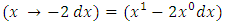is , which yields the exact arm 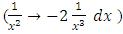. This simple procedure for finding the rectifying factor r₃ when the -arm extends between power functions of x with exponents differing by unity, will be applied in [part C] repeatedly. The rectifying factor r₃ multiplies the two functions of the independent arm to turn it exact without disturbing the exactness of the dependent arm. It also multiplies the non-homogeneity term without disturbing its being a singlet (individually integrable), since the two are functions of the same single variable. The second part of the table applies to certain equations with second order doublets (see Example 6].

2. Seven Semi-exact Equations of Different Types Quoted with Their Prolonged Solutions by the Current Methods, and Reworked by the Much Shorter and Simpler Methods of Test-by-sight and Integration by Parts

Example 1: Bernoulli’s equation as a typical semi-exact equation with a two-variable integrating factor obtainable by the three-rectification test-by-sight and not by partial differentiation. Derivation of a readily applicable formula. The multiply-integrate-and-divide formula

Bernoulli’s equation 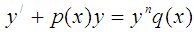is a three-term equation identifiable by sight. This equation is amenable to the three-rectification process, i.e., to finding the factors by sight thanks to its having two unique properties: (1) The non-homogeneity term is the product of two factors comprising the two variables x and y separately. This property makes it possible to turn this non-singlet, simply by division, into a singlet (individually integrable by the basic formulas). (2) The functions of the three y’s in the non-homogeneity term and in the dependent arm are “power functions”. In the linear arm we note that is to the first power, and is multiplied by y to the zeroth power and the difference between the exponents is unity (1-0 = 1) which remains unchanged and thereby keeps the semi-exactness of what will be a non-linear arm after multiplying the equation by . Instead of solving Bernoulli’s equation by the usual substitution and repeating the calculation every time, a ready formula can be derived by carrying out the three rectifications . 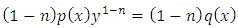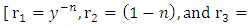The equation will then become:

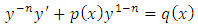⇒. The y-arm is now exact . The individual integrability of is not disturbed by the constant factor . The exact linear arm is first turned semi-exact non-linear, then exact non-linear. Finally we have a semi-exact x-arm: for which the integrating factor is . Thus we obtain: which is an exact equation, i.e., with a doublet reciprocating two exact arms. Recalling that the integral of an exact doublet is equal to the product of the outer functions of the doublet, we obtain:

(multiplying by ): (raising to the exponent ): , which is the “general solution of Bernoulli’s equation”. At first sight the equation may appear to be difficult to memorize. However, this difficulty can be overcome by the following wording: “to solve Bernoulli’s equation, multiply the rectified non-homogeneity term by the integrating factor , integrate, and then divide by the same factor. This “three-step multiply-integrate-and-divide method” is an inner component part to be complemented by multiplying by and raising to the exponent ”. It can be seen that: (1) All the semi-exact three-term equations with two variable integrating factors (i.e., with non-singlet non-homogeneity terms) can be turned by factor (r₁) into equations with one variable integrating factors (i.e., with singlet non-homogeneity terms). (2) What we have called “multiply-integrate-and-divide method” applies “after” multiplying the equations by (r₁ and r₂). This method is concerned only with (r₃) which appears twice: inside the integral signs where it “multiplies” the rectified non-homogeneity terms and forms new integrands, and outside the integral signs where it “divides” the results of the integrations. That is simply what is denoted for brevity by the newly introduced term “multiply-integrate-and-divide formula”. It simply means that the solution of the non-linear semi-exact equations with singlet non-homogeneity terms, and with exact dependent arms, i.e., with is expressible in one direct step by the readily applicable formula: . This is actually the formula preceding the general solution formula above.

Note that the general solution formula derived for Bernoulli’s equation is a function of x alone, and in it r₃, , and are readily obtainable by sight. This formula reduces the solution of Bernoulli’s equations to the simpler problem of solving one integral whose integrand is the product of two functions of x.

Example 2: A semi-exact equation in differential form solvable by separation of the variables by substitution and by integration by parts:

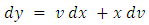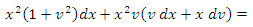
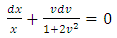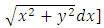
(A): We put then and the given equation becomes: . . (separating the variables). Consequently, the solution in terms of . Hence, using each member as an exponent of e, we have and, replacing , we get . The form of the solution can be modified by removing parentheses. Thus, we find that is the general solution][1].

(B): A differential equation is presented either in differential form as in this example or in derivative from as in the next example. Where the equation is presented in differential form we should cease to collect the like differentials on and separately. Instead, we should identify by sight which differentials are singlets (individually integrable), and which are non-singlets, and whether the latter constitute one or more doublets integrable by parts, or can be made so by an integrating factor that is also obtainable by sight”.

The first step of the solution is to rearrange the given equation by putting the doublet on the left side of the equation and the non-homogeneity term on the right side: In applying the three-rectification process mentally we find that the non-homogeneity term is a singlet (i.e., in an already rectified form whose rectifying factor is r₁ = 1). The is semi-exact (extending between power functions of y with exponents differing by unity) and its rectifying factor is r₂ = 2, thereby obtaining the exact dependent arm . The independent arm is initially exact but has been turned semi-exact after multiplying by 2. It can be returned exact again by multiplying the equation by rectifying factor r₃ = and obtaining . After such mental analysis we conclude that our equation is semi-exact having as its three rectifying factors. The second step is to multiply the equation by the total integrating factor to become exact: . The brackets are meant to help the reader to identify the reciprocated arms between the two terms of the doublet, and when sufficient skill has been gained then such brackets can be dropped. The doublet is now the differential of a product, . The third step is to integrate the equation by the pair-wise and term-wise integrations and get: , as in (A) above. Again, compared to the prolonged solution by the method of substitution and separation of the variables in (A), the considerably shortened three-step solution by the methods of test-by-sight and integration by parts in (B) may seem magical. The solution avoids the details of substitution and back substitution, solving the corresponding homogeneous equation,…The equation is a nonlinear, non-homogeneous, first-order equation with variable coefficients. We remind that, except for the three steps of the solution, the detailed writing above is for explaining the unwritten mental test and constitutes no part of the written solution.

Example 3: A semi-exact equation in derivative form solvable by separation of the variables by substitution and by integration by parts.

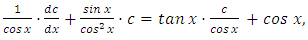
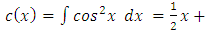
(A): [Solve the equation: . Solution: the corresponding homogeneous equation is Solving it we get: Considering as function of , and differentiating, we find: Putting and into (…) we get: Whence Hence, the general solution of equation (…) has the form

(B): Checking mentally the possibility of the equation being semi-exact (i.e., possessing an integrating factor and solvable by integration by parts) we find: firstly, the rearranged equation has a semi-exact doublet with the exact y-arm and the semi-exact x-arm and we thus have as the required integrating factor [recall that r₃ for , which yields the exact arm . Secondly, we multiply by this factor and obtain 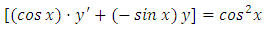which is now an exact equation reciprocating the arms or whose doublet is the derivative of a product . The non-homogeneity term becomes after multiplication by the integrating factor and its being individually integrable remains unaffected by such multiplication since the integrating factor is a function of alone. The integral of the exact doublet is the product of the outer functions of the doublet and is a tabular integral. Thirdly, we integrate and get: as in (A) above. We can also apply the three-step multiply-integrate-and-divide formula 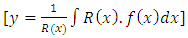and obtain the same result in “one direct step by this readily applicable formula” followed by applying the tabular integral. The methods in (A) of solving the corresponding homogeneous equation for finding the complementary function and of using variation of parameters for finding the particular integral have become a past history. They are no longer practical and have to leave their places to the short methods of testing by sight and solving by integration by parts as in (B) (as far as exact and semi-exact equations are concerned). Again, we remind that the writing above is mainly a description of the mental (unwritten) analysis of the problem and of the traditional methods dispensed with, and that the solution in (B) is much shorter and simpler than in (A).

Example 4: A multi-term equation with two semi-exact doublets requiring the same integrating factor (derivable by partial differentiation and by the three-rectification test-by-sight)

(A): [Solve the equation: . Solution: Here and 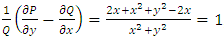, hence, Since , or 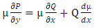, it follows that 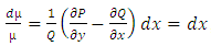, and 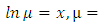Multiplying the equation by , we obtain 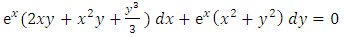which is an exact differential equation. Integrating it, we get the general integral 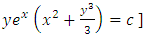[2].

(B): It is obvious that the quoted solution concentrates on establishing the semi-exactness of the given equation and determining its one-variable integrating factor by the method of partial differentiation. It does not mention the prolonged method of solution applied (i.e., integration in total differentials) leaving it to be impliedly understood for the sake of brevity. Let us also note that an exact triplet of terms can be reduced to an exact composite doublet reciprocating one composite and one simple arms: with the exact composite arm and the exact simple arm . The given equation is not a three-term, but a five-term equation. However, subjecting it to test- by- sight for establishing its semi-exactness and obtaining its integrating factor is still possible though not as easy as before. It actually requires some more skills to be gained since it is not so similar to the previous examples but possesses the following dissimilarities:

In attempting to distribute the terms of the given equation among the defined combinations of terms it will be seen that three non-singlets out of the five terms of the equation 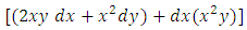constitute a semi-exact composite doublet having an exact composite arm 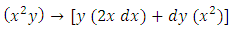and a semi-exact independent arm requiring the integrating factor to become exact .

Of the two remaining terms the singlet y²dy will not be integrated individually, (contrary to what we usually do), since the other non-singlet would then be floating outside the combinations leading us nowhere. It can be seen that these two terms constitute a second semi-exact simple doublet 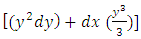with the exact y-arm and the semi-exact x-arm that requires the same integrating factor to become as in the first doublet. Having performed our mental analysis (i.e., having rearranged the terms of the given equation in a first step, and found the integrating factor by sight) we then take the second step of multiplying this semi-exact equation by its integrating factor and obtain it in its exact form. 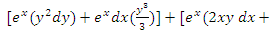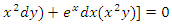. 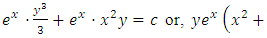Recalling that the integral of an exact doublet is the product of the outer functions of the doublet, we apply the one-step integration by parts as the third step, and obtain , as in (A) above. It is also noted that if to this five-term equation a sixth singlet term is added as a rectified non-homogeneity term, the equation will still remain integrable in the same manner since the individual integrability of the added term will not be disturbed by multiplication by the integrating factor.

The solution in (B) is by far shorter and simpler than that in (A) which employs prolonged methods for determining the integrating factor by partial differentiation and for integrating in total differentials (not mentioned in the quoted solution in (A), obviously for brevity, and assuming the reader to be familiar with it).

NOTE: The following three examples have been postponed to the next paper so as to avoid the present paper becoming excessively lengthy.

Example 5: Semi-exact first order equations (linear and non linear, with constant and with variable coefficients). Applications from classical mechanics and nuclear physics

Example 6: Equations with semi-exact second order doublets (an application from quantum mechanics-Schrödinger’s equation)

Example 7: Generalization of the solution of the semi-exact linear equation with constant coefficients to the n-th order case by a readily applicable formula

3. Practicing the Test-by-sight for Establishing the Semi-exactness and Determining the Integrating Factors of Miscellaneous Semi-exact Equations. [2, 3]

Semi-exact equations with two-variable integrating factors are not so frequently encountered in the literature, and if they are ever encountered (such as Bernoulli’s equation) then they are solved by such prolonged methods as that of separation of the variables by substitution without realizing the integrability of the equations by the integrating factor method (i.e., by integration by parts). The two-variable integrating factors cannot be derived by partial differentiation which is the only method known so far (before the newly introduced test-by-sight method) and is restricted to the case of one-variable factors only. Solution of the n-th order linear equation with constant coefficients by using “n integrating factors in n successive integrations by parts” will be dealt with in the next paper. Examples of equations with two-variable factors derived by sight are already given in [part A-4-b]. This part C of the paper concentrates on semi-exact equations with one-variable integrating factor (either r₁, r₂, or r₃) that rectifies only one of the three constituents of the equations below. The two other constituents are either initially given in rectified forms, or created or rectified subsequently by the first rectifying factor r₁ itself. The below mentioned equations are meant by their references for practicing the determination of integrating factors by the partial differentiation method and solving by integration in total differentials. We shall, however, replace these prolonged methods with the much shorter and simpler test-by-sight and integration by parts. If an equation is given in differential form, we disregard the collection of the terms on like differentials and rearrange them often with the singlet and non-singlet non-homogeneity terms put on the right side (unless otherwise is required for constructing doublets in certain cases) and the doublets on the left side of the equation, and thereby perform the first introductory step for rearrangement of the equation. After rearrangement of the given equations the three rectifying factors become readily determinable by sight in the order: r₁ for the non-homogeneity term, r₂ for the dependent arm, and r₃ for the independent arm. As already mentioned factor r₂ is determined after multiplying the equation by r₁, and factor r₃ after multiplying by r₂. The second step is to multiply the semi-exact equation by the one-variable integrating factor to turn the equation into the exact form. The third step is to integrate the resulting exact doublets by parts, and the singlets by the basic formulas. This new method of solution by integration by parts is by far superior to the traditional method of solving by integration in total differentials, in terms of the space, time, and mental effort expended on the solution.

Greater attention and concentration may have to be exercised in solving the following semi-exact equations by applying the short methods of the “three-rectification test by sight” and “integration by parts”.

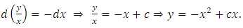
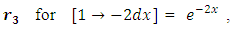
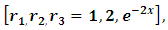
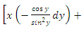
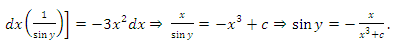
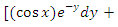
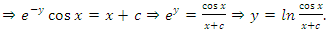
(two semi-exact doublets requiring the same integrating factor,

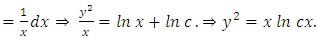
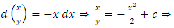
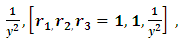
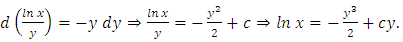
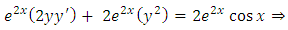
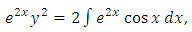
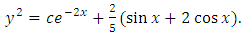
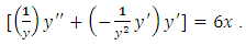The first integration is .

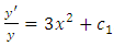4. Conclusions

In semi-exact equations the three rectifying factors are determined by sight to constitute one-variable, or two-variable integrating factors that turn these equations into exact ones. The table of integrating factors is intended for general acquaintance, is easily memorized, and can be extended further. Semi-exact equations are solvable by the three methods of separation of the variables, integration in total differentials, and integration by parts, of which the last is the most convenient and the first two are no longer required, having become unnecessary prolongation as far as exact and semi-exact equations are concerned. It must, however, be stressed that the separation method retains its importance in solving the separable non-exact equations to which integration by parts is inapplicable and the separation of the variables is the only applicable method. Finally, the previous and present papers will serve as a basis for revising other related topics to be handled in forthcoming papers.