Branko Mišković
Independent, Novi Sad, Serbia
Correspondence to: Branko Mišković, Independent, Novi Sad, Serbia.
| Email: |  |
Copyright © 2016 Scientific & Academic Publishing. All Rights Reserved.
This work is licensed under the Creative Commons Attribution International License (CC BY).
http://creativecommons.org/licenses/by/4.0/

Abstract
Instead of material particles, as the field sources or carriers, we start with EM potentials, as the energetic medium disturbances. EM fields thus appear as formal features of the potentials, and carriers – of these fields. The fields and potentials may move with or without apparent carriers. Their variations, caused by motion of their non-homogeneities, are finally expressed by the temporal derivatives. Two algebraic relations of J. J. Thomson are thus directly interrelated with Maxwell’s differential equations. Instead of parallel treatment of two EM fields, the static, kinetic and dynamic EM processes, dependent on mutual position, separate motion and acceleration of two electric polarities, are finally arranged into the causal loop. All EM quantities, and each equation relating them, are interpreted by respective processes in the medium. Not only that the new interpretations explain physical essences of all EM phenomena, but the new formal relations resolve some former problems and enable additional applications of EM theory.
Keywords:
EM theory, Formulation, Interpretation, Elaboration, Exposition
Cite this paper: Branko Mišković, Elaboration of Electrodynamics, International Journal of Theoretical and Mathematical Physics, Vol. 6 No. 1, 2016, pp. 31-42. doi: 10.5923/j.ijtmp.20160601.03.
1. Introduction
1.1. Former Bases
In the originally founded mechanics, Newtonian laws treat the motion and balance of usual solid bodies, reduced to the material points situated in their centers. This initial set may be supplemented by the law of gravitation, as the static interaction of two massive bodies. Such foundation of electrodynamics is reduced to Coulomb’s law of the static interaction of two electric charges. Attempting to express the analogous force between two moving charges or elementary currents, Ampere failed to obtain its general form, owing to the vague fields and their motions.For description of physical processes in space and time, the formal field theory is developed and consistently applied to mechanics of fluidic and solid bodies. As such, it has not been extended to the invisible EM fields and their uncertain motions. Irrespective of accepted fields, their motions were not even supposed, let alone – formally treated. The theory is founded on electric circuits and their interactions. Instead of the field motion, their variations are observed. The algebraic field relations are thus bypassed, with the ready differential notions taken from fluid mechanics. Though unilateral, EM theory is applied in practice, and its incompleteness is not noticed. The faults were manifest at the attempts of its application to micro-structure. Instead of its further elaboration, this theory is pronounced incompetent for this purpose. It is then substituted by a sequence of the particular, less consistent, modern theories. Instead of some reduction of physical quantities and the laws relating them, they are further multiplied or complicated. In the absence of clear visions of physical processes, their mutual relations are subordinated to ideal formal principles.
1.2. Consistent Elaboration
Via relation of temporal variation with spatial motion of EM fields, a few their algebraic relations are reaffirmed and compared with standard differential equations. Instead of the material particles, as the sources or carriers of their fields, these particles are found as the formal features of the fields, and these fields themselves, similar features of the potentials. These potentials represent respective energetic disturbances of the vacuum medium, as the ambient of physical events. With consistent reinterpretation of the theory, a few inherited fundamental problems are resolved.Thus elaborated EM theory is here convincingly exposed. It appears equally applicable to final explanation of the laws of mechanics and of micro-phenomena noticed empirically. The inertial mass, its function against motion and defect in compound structures are finally reduced to EM processes around elementary particles. However, with respect to the main orientation to the theory elaboration, as the systematic formulation and presentation of its equations, such details are ceded to the paper [1]. These two scientific approaches just supplement and support each other.Carefully built and continually reconsidered, the former gradual elaboration of electrodynamics [2] started from the two assumed EM carriers and persistent exploiting of their symmetries. Though successfully surpassed or limited, these procedures considerably charge that detour exposition, by some excessive procedures clouding physical essences. This brief deductive exposition concerns the final essence and its convincing argumentation, without excessive concepts and procedures. The more detailed former text [2] presents the initial gradual inductive elaboration.
1.3. Starting Views & Conventions
In the aim of this deductive exposition, a number of the starting views and conventions is adopted. Apart from space and time, as the formal frame, some vacuum medium, as the ambient of physical processes, is indispensable. Although denied in some speculative theories, certain features of this medium are manifest by a sequence of natural phenomena. With respect to its polarization and transfer of EM waves, this is a dielectric medium, very similar to usual matter. The energetic disturbances of its much finer structure may be the final essence of all physical events. 1The polarization is opposed by the strains of the deformed structure. Its elasticity (εo) determines the static state of the medium, manifest by the electric quantities. On the other hand, the bound electricity is expected to be inert, in accord with respective mass density (μo). This feature determines its motion, allowed by the elasticity and manifest by magnetic quantities. In the presence of some material media, these two features are scaled by the relative factors:  Thus interpreted, the two constants typically determine the speed of wave propagation: c2 = 1/εμ. 2 At vacuum, as the etalon medium – with the unit relative, the constants reduce to the vacuum factors. Their numerical values depend on the units of the quantities related by them. In natural system (NS) the vacuum factors are adopted as dimensionless units. The speed of wave propagation through material media is diminished and determined by the relative factors. Operating by the symbols of the vacuum factors, the measuring units are irrelevant. 3 As an additional convention, discrete physical quantities are here denoted by lower cases, and distributed – by respective capitals.
2. Formal Field Theory
In the simplest physical relations – of the mechanics, the volumes and possible deformations of interacting bodies are neglected. Their dimensions and all other features, as their masses or speeds, are thus reduced to their centers. In some practical situations, two or one dimension may be abstracted, observing the quantities as the line or surface fields. In the general case, of the mechanics of fluidic and solid bodies, the discrete quantities are treated as respective physical fields distributed in 3D space. This exposition of EM theory will be gradually extended into 4D space.Discrete substantial quantities, as mass or electric charge, represent respective integral sums of the continual fields, as the distributed quantities. The return to the fields thus uses the volume derivatives of these quantities. In the statistical approach, these fields are defined as the local concentrations of respective particles, as small discrete bodies. In both these cases, the transfer into fields includes dimensional division by volume. Volume derivative of the fields themselves equal to zero, i.e. they behave as the constants in this procedure, directed along the structural depths.Kinematical quantities observed in 3D space directly turn into respective fields, of the same dimensions. As the vector quantities – of the distributed intensities and directions, their cross-sections are presented on the drawings by the oriented curve lines, so that the line density illustrates field intensity. Rational fields, obtained by multiplication of the kinematical and substantial, are equally presented. The originating fields are expressed by terminated, and vortical – by closed field lines. These features are expressed by the spatial derivatives: origination  and circulation
  These two are related with the gradient (∇), expressing the field variation in space. Applied to a scalar field, it gives the vector determining its dominant slope. Projected into other directions, it is the scalar quantity. The gradient applied to a vector field gives the tensor, as the set of derivatives of all components per each axis. Scalar product of this result and a new vector gives also the vector. Its values thus depend on vector features of the multiplier. Such are the relative and convective derivatives (1), with respect to the speeds applied: of the object (v) or the field itself (V).
  | (1) |
The former of them, concerning a moving object, is of the same sign, and latter is opposite to the field gradient, with respect to the speeds applied. These two derivatives manifest as the temporal field variations on the object independently moving. At their common motion, this result annuls. Thus being additive, these two derivatives are mixed or unified, especially in EM field theory. Apart from their opposition, these derivatives are defined in the distinct domains. The former is restricted to the object volume, and latter of them concerns the whole field domain.Longitudinal gradient is wider from the field origination, for divergence of the field lines. Though electric field lines diverge in the space around a central charge, their origins are restricted to the charge itself. Similarly, with transverse field gradient, the curls of its lines contribute to field circulation. The gradients and curls of the magnetic field around a line carrying conductor annul, thus reducing the circulation to the current itself. Therefore, at uniformly moving fields at least, the origination accords with longitudinal, and circulation – with the transverse field gradients. 4The force fields are usually introduced directly. A medium pressure, as the volume density of energy, represents a scalar field. The surface field of height expresses the ground relief. The negative gradient of this field, directed down the slopes, is related with gravitational forces, as the originating field. Its field lines start on the hills, and terminate in the valleys. They are expressed on maps by the perpendicular isohypses, as the vortical field of the equipotential lines. Instead of the opposite curve orientations on the hills and valleys, they are distinguished by distinct backgrounds.A vector field integrated through a final surface gives its respective flux. The flux of an originating central field around a pole is distributed about concentric spheres, and so, the field obeys inverse square function. Mentioned spheres represent the equipotential surfaces in this field. However, the axially symmetric fields obey the simple inverse function. The flux of a transverse (line-originating) field is distributed about coaxial cylindrical surfaces. Circular cross-sections of the equipotential surfaces of such a longitudinal field are presented by the oriented isohypses.
3. Static Interactions
3.1. Static Equations
Alike the mechanical pressure disturbances, opposed by deformed medium structures, the vacuum medium stressed by electric potential pushes out the object charge of the same polarity, but sucks the opposite. As if that the object charge itself tends to the minimal its own energy. In other words, it is affected by electric force field, as the negative gradient of the static potential (2a). The potential and field are associated with a polarity of the assumed electricity. The usual inverse equations form the sequence defining EM quantities, from the potential up to electric charge:  | (2) |
The medium polarization is proportional to the force field and elasticity (ε) of the medium structure (2b). This field means the relative displacement of the positive, with respect to negative polarities: D = QoR. The terminals of this field compensate the opposite surface charge (2c), expressed by respective volume density: Q = ∂q/∂v. Introduced as a formal concept, it was the starting quantity in the former theory. The opposite sequence was terminated by the potential, as the energetic feature of the field. Our sequence starts from the energy, as the final essence: W = QΦ.
3.2. Central Fields
Above mutual relations of the static fields determine the central field distributions (3). Radial derivative of the static potential gives respective field, with the full flux of electric displacement equal to the carrying charge (q). The reaction of the medium, by some displacement of its own electricity, compensates the disturbances of material charges. This fact accords with their 4D relations: the potential – axial to the t-axis – obeys the simple, and the field – centrally symmetric in 3D – obeys the square inverse functions. These facts just accord with their formal relations. | (3) |
The static force acting on an object charge, f = qoE, can be further generalized. The charge inserted into metallic sphere attracts the opposite, and repels the same structural polarities. The former effect compensates the inserted charge, and latter one forms outgoing flux of the displacement, thus polarizing surrounding medium, including the spherical metallic walls. Discharging the external polarity, Faraday established its strict equality with inserted charge. The general neutrality of each 3D location results from the opposite disturbances of the two (or more) structural strata.
3.3. Bipolar Objects
Two opposite electric charges, somehow connected at a distance r, form respective dipole: p = qr. Acting by opposite forces upon the two poles, foreign electric fields manifest by the torque and force difference (4) affecting the dipole, as a whole. The torque directs the dipole in the field course, and the force pulls already directed dipole into the domain of the stronger field. The foreign fields also polarize the neutral material scrapings, forming respective dipoles. Their chains illustrate the abstract field lines, as the empirical suggestion for the graphical field presentation. | (4) |
Neutral structures, as atoms, do not manifest their electric features. However, the foreign fields displace the centers of their opposite charges, thus forming the dipoles. This means that their opposite electric fields exist in parallel, displaced energetically along the structural depths. Irrespective of the general neutrality, various medium strata are charged by the opposite polarities and energy densities. The opposite forces of the disturbed strata form the action-reaction pairs. Their summary balance points to the total energetic homogeneity, as the most general physical law.
4. Kinetic Interactions
4.1. Kinetic Quantities
A moving charge forms electric current (5), and moving static forms the kinetic potentials (6), collinear to the current. Unlike the former simple definition, the latter includes the two constants. The static potential, as a pressure disturbance, multiplied by medium elasticity (ε) and density (μ), gives the density disturbance. Its motion forms the kinetic potential, proportional to the linear momentum density. Owing to their inertias, the fields are moving uniformly. Spatial derivatives thus annul, and convective ones remain. The two definitions thus give the continuity equations (b). | (5) |
 | (6) |
Unlike the simple current definition, that of the kinetic potential, a little more complex, has not been used so far, let alone – thus precisely interpreted. Apart from the acceptable motion of the concept of electric charge, such motion of its potential could not be even imagined. However, respective continuity equation (6b) was introduced intuitively by L. Lorentz, and widely accepted as a formal condition. It is here derived and interpreted. The moving static potential, as the energetic medium disturbance, is followed by the electric charge, as its secondary characteristic. 5
4.2. Kinetic Equations
Two parallel, mutually related magnetic fields are defined by the kinetic sequence (7). With respect to definition (6a), their equivalence is confirmed in (8). The force field (B) is proportional to the density and kinetic disturbance (H) of the medium, as the rational field. Both these fields just express cylindrical equipotential surfaces of the kinetic potential, by the field lines, as the isohypses on transverse cross-sections of these surfaces. In the simplest case of a line current, these lines are the embracing concentric circles. A moving electric thus produces magnetic fields (7c). | (7) |
 | (8) |
Though noticed by J. J. Thomson, in the absence of clear interpretations of EM fields and their motion, (7c) is usually ignored. However, its circulation gives the kinetic Maxwell’s equation (9). As before, the spatial speed derivatives are missed. In accord with the static equation (2c), the former term represents conduction and/or convection current of the free electricity. As the convective derivative of the electric displacement, the latter term represents the current of bound electricity – through dielectric media, including the material and vacuum strata of their structures. | (9) |
The origination of the magnetic field (7a) gives the trivial Maxwell’s equation (10). The mixed vector product with one repeated factor (∇) here annuls. In the partial symmetry of Maxwell’s equations, this one is of magneto-static sense, as the pandanus of the static equation (2c). In the formal sense at least, respective magnetic charge was expected. However, the trivial equation (10) explicitly points to the absence of any originating magnetic field and respective free charge. With respect to the field lines, as the isohypses of the kinetic potential, they are ever closed curves. | (10) |
In accord with the static and kinetic fields (6,7), a moving punctual charge with its two static fields (3) forms the two kinetic fields (11) respectively distributed. The longitudinal potential is followed by circular magnetic field, with respect to the motion. These two are the same inverse functions of the radius, as (3) are, with the new dimensions of speed, and – addition or reorientation – of the vector form. Owing to the vector product, magnetic field is the sine function of polar angle, between the two vectors. The distinct motions of the two fields will be determined soon. | (11) |
Substituting the algebraic (7c), by the differential equation (9), the kinetic sequence is fully analogous to the static one (2). The current of free electricity (5a) is extended by the displacing of the bound medium electricity (9). The parallel equations result from the definitions (5, 6, 7) of the kinetic, by motion of static quantities. Thus distinct by their respective interpretations, they may be also located on respective two structural strata or the levels of considerations. In fact, the static quantities – in their own motion – are supplemented by addition of respective kinetic energy.
4.3. Kinetic Fields
Unlike static forces – collinear with electric field, kinetic forces are to be related with magnetic field. With respect to the indirect field sense, these forces are more easily related with the current and kinetic potential. As the known kinetic effect between two fluidic flows, we consider the mutual interactions of line carrying conductors. Owing to reduced transverse pressures, two parallel currents mutually attract. Two opposite currents form the potential vortices in between, moving apart the two conductors. Both these causes rotate crosswise currents into the same course.These interpretations are expressed by the three functions of kinetic quantities (12). The kinetic forces are presented by equivalent static quantities. The speed (v) concerns the static objects moving through the kinetic fields around respective current. Though agree with the middle, two external relations are not general. The two scalar products concern longitudinal motion only, unlike the vector product treating the transverse motion too, also perpendicular to the circular field. This is a formal justification and the first practical advantage of the magnetic field introduced indirectly. | (12) |
This sequence is a formal inversion of the three definitions (5a,6a,7c). 6 Apart from the opposite course of speed, the two constants are replaced from the potentials to the carriers. At motion through 3D space, these relations express the axially symmetric, line-originating, electric field. The first of them announces an additional result. At some speed v = c – along temporal axis, the transverse result – from 4D, is projected into – centrally symmetric – 3D value: Φ = – cAt. In fact, this simple result points to the effect of static potential, at motion through the opposite kinetic flows.At motion of conducting matter through magnetic field, its free electricity plays the role of the moving object charge. The kinetic forces (12b) are manifest as respective induction. Let us observe two perpendicular object conductors, one of them parallel and other perpendicular to the current carrying conductor. At transverse motion of the object conductors, respective longitudinal inductions are obtained: vortical – in parallel, and line-originating – in perpendicular one). In the former case, the effect is additive with the dynamic induction, at motion of the carrying conductor.In the latter case, the equivalent electric field and static potential are reduced to the object conductor and its motion. The equivalent charge may be imagined on the carrying conductor. Faraday obtained just such radial induction in a conducting disc rotating in the front of a cylindrical magnet. The induced ‘electric’ field is reduced to the disc volume. The equivalent charge belongs to the magnetization current, situated on the magnet cover. This kinetic interaction cannot be anyhow reduced to the classical formal concepts and soon interpretation of the dynamic induction.
4.4. Kinetic Force
The mere substitution of (11b) into (12b) gives the kinetic force (13), consisting of the two terms, dependent on the object motion in a longitudinal plane. Its circular motion, along the magnetic field, would not produce any effect. With respect to the inverse square function and sine dependence on the polar angle, both components are some combinations of the central and cylindrical forms. The longitudinal force component is unidirectional, irrespective of the polar angle. At the two parallel motions, the kinetic force (13) is reduced to its transverse component (14). | (13) |
 | (14) |
Acting in return to its own field carrier, the force at left (14) maintains the rectilinear motion. Its torque as if exerted on a moving dipole is compensated by the longitudinal dynamic forces (20). The case of the common abreast motion of all material existence along temporal axis (v = c = – V, sin θ= 1) is presented in continuation of (14). The speed v concerns the cosmic expansion, 7 and V – opposite kinetic flows around the particles. The static thus appears as the special case of the partial kinetic force. The transverse direction – around t-axis, is manifest as radial – in 3D space.The transverse validity of this law enables its application to parallel conductors. The unit of line current is thus defined. With respect to the circular magnetic field lines around a line current, the field of a current loop is in the toroidal form. Its internal flux plays the role of the magnetic moment or dipole. Unlike electric dipoles, which fields start from the positive, and terminate on negative apparent poles, magnetic poles are transparent for respective field. Nevertheless, at foreign magnetic fields they suffer the torques and force differences (15) in the same forms of that in (4). 8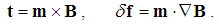 | (15) |
In the technical practice, magnetic moment is defined as the product of the loop current and the surface embraced by the loop. This definition accords with the usage of the sector speed, at planetary orbits. With the double angular speed, the magnetic moment is better defined by rotation of an electric dipole around one of its two poles, m = qr v, giving the double value of the moment. Similarly to electric, magnetic field magnetizes respective material scrapings. Their chains announce the magnetic field lines. The effects (15) were the empirical bases for the field introduction.
5. Dynamic Interactions
5.1. Dynamic Equations
Apart from the kinetic induction, arisen at the transverse motion of object conductors in the field of a carried current, the same motion of the carrying conductor gives the opposite effect, described by Thomson’s dynamic relation (16a). Here U denotes the motion of the current with its magnetic field. The addition with kinetic induction (12b) formally unifies the two results (16b). Using the mutual speed, v' = v – U, the principle of relativity is introduced, thus avoiding the strict determination of the reference frame. Relativistic views were initialized by this artificial synthesis. 9 | (16) |
Circulation of (16a) gives Maxwell’s dynamic equation (17a). With zero origination of the vortical magnetic field – in the latter, the former term represents the convective field derivative. The field moving along its own gradient results in its convective variation in the resting points of the medium, with respective induction. In accord with the definition (7a), the induction is more directly related with kinetic potential (17b). With respect to the definition (6a), announcing linear momentum density, this is nothing else but force action law (18), expressed by the fields. | (17) |
 | (18) |
The procedure (17a) shows some physical restrictions of the synthesis (16b). The two thus unified interactions are also distinctly limited. Unlike the apparent kinetic field, restricted to the moving object conductor, the real dynamic field is manifest in the whole domain of the moving magnetic field, unlimited in space. Moreover, unlike the kinetic induction, obtained at any object motion perpendicular to the magnetic field lines, dynamic one is restricted to the field gradient, in the planes of the field lines. Axial motion of the carrying conductor does not produce any effect.The equations (17) were initially introduced as induction established by Faraday. At some accelerated motion of the free electricity along a line conductor, the increasing kinetic potential causes the opposite longitudinal induction (17b). This fact is manifest as the voltage in all parallel conductors, including the carrying one. The two effects are known as the induction or self-induction. The circular magnetic field also grows in this process, thus expanding transversely, with the same effect (16a). Of course, at the decreasing current and magnetic field, the effect is opposite.
5.2. Dynamic Force
Not only that kinetic potential is produced by motion of static one (6a), but it itself also moves at the same speed (V). However, this speed cannot bi ascribed to the magnetic field, as the formal consequence of the moving electric field (7c). Defined by (7a), as circulation of elementary potential (11a), respective magnetic field (11b) is reduced to the transverse gradient or respective convective derivative of the potential. With respect to the circular cross-sections (ρ2 + z2 = r2) of the potential, and their derivatives (∂ρ/∂z = –z/ρ), the transverse magnetic field speed is obtained (19). 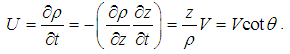 | (19) |
This process is illustrated on the Fig. 1. The longitudinal motion of the potential is followed by transverse contraction of respective magnetic field. Its field lines expand in the front, and shrink behind the moving charge. As if that the longitudinal particle motion is enabled or even determined by the transverse contractions of respective magnetic field. Unlike the particle motion, limited by the speed of light (c), the field contractions tend into infinity around the axis. This fact is possible due to the formal sense of the magnetic field, unlike respective essential potential. 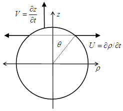 | Figure 1. Moving central fields |
With thus obtained motion of the magnetic field (11b), the dynamic relation (16a) just determines respective force (20). On the other hand, Maxwell’s equation (17b) applied to (11a) would give the same result. Being independent of the object motion, this force is not of kinetic, but of dynamic natures. The symmetric longitudinal force is directed to the moving particle, from both its axial sides. Subtracted from the radial static field, it causes its ellipsoidal deformation. Towards the speed c, the charge is reduced to the ratio 2/3. Both these effects were already somehow predicted. 10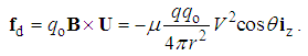 | (20) |
The two opposite axial forces are equal at uniform motion. This ahead predominates at acceleration, and that behind – at deceleration. Both effects manifest as the induction or inertia (18). In any case, they may be interpreted by the compression and acceleration of the medium electricity – ahead, and the opposite processes behind the moving charge. As such, they also affect all the surrounding charges. These processes in complex structures are restricted to the space between the particles, and manifest mechanically. Material inertia is thus reduced to the same medium feature. 11
6. Unity of EM Fields
6.1. Speculative Unification
Summary force of the two EM fields exerted on a moving charge is expressed by the equivalent field (21a), observed in the moving frame. The principle of relativity understands the mutual speed of the electric object and magnetic field, and so the kinetic and dynamic inductions are added to the present electric field. The similar magnetic force would understand the free magnetic poles, affected by some equivalent field (21b). In the absence of the free poles, the forces acting on respective dipoles are restricted with respect to the expected limitations of their motion and effects. 12 | (21) |
These two transformations can be formally inverted (22). With the opposite speeds or inductions, the new equations are also scaled by the set determinant, g2 = 1 – εμv2, pointing to preferential status of the frame connected to the medium. Denying the invisible vacuum medium, the set determinant is divided between the two sets, by 1/g in each of them, with conservation of mutual inversion. According to the relativity, the increased – here relevant – transverse fields (21) may be equivalent with reduction of the longitudinal electric field, caused by the dynamic induction (20).  | (22) |
This deformation of the transverse fields calls in question Maxwell’s equations. In the aim of their form covariance, the longitudinal and temporal axes are inversely transformed. In the causal sequence, each former – is tried to correct by the next inconsistencies. These formal procedures can be neither followed intuitively, nor their results rationally interpreted. The space-time relativity calls in question the formal frame of any consideration. In the final instance, our exposition does not depend on this speculation. In the unique space and time, all the procedures are consistent.
6.2. Essential Unification
Sum of the static (2a) and dynamic (17b) electric fields as if forms the vortex of the kinetic potential in a ‘longitudinal’ (tr)-plane (22). As being expressed in the vortex plane, this is the polar vector, unlike magnetic field axial to the vortices in the ‘transverse’ planes – of 3D space. This formal distinction is sometimes mentioned, but without any needed explanation. The essential unity of the three EM fields (static, kinetic and dynamic) is thus established. However, the clear distinction of the native planes explains the exclusivity in the experience of the electric and magnetic forces. | (23) |
Equal treatment of the two axes understands NS, with the same dimensions of the two potentials: –Φ = cAt (=) At. This equality points to the positive potential, as the result of the negative flows around a positive particle. The vortices (23) form respective magnetic field omnidirectional in 3D space, and so – usually unmanifest. However, with respect to the dynamic relation (16a), their axial motion just produces the radial – static field. The same statement is also expressed differentially (24a). The causal sequence of all EM processes is closed by the static equation (24b). | (24) |
The usual implicit unity of EM fields was intuitive, only supported by their causal relations, in Maxwell’s equations. Not only that these relations are now explicated and further confirmed by the algebraic equations, but the causal loop of EM processes is finally closed. In this aim, the two electric fields, static and dynamic, are technically distinguished. The magnetic forces are then conveniently expressed by the three equivalent static quantities. The causal loop is closed in 4D, by axial temporal motion of magnetic vortices. Static field is obtained as the projection into 3D.
7. Basic Equations
7.1. Constitutive Relations
The two constants in (2b&7b) were already resolved into their vacuum and relative factors, ε = εoεr, μ = μoμr, as such interpreted by the media stratification into the vacuum and material strata. However, the constants are defined distinctly (25, 26). Apart from inverse senses, internal fields of electric and magnetic dipoles are opposite: the former subtract from the total, but latter add to the vacuum fields. Thus the electric forces accord to the full medium disturbance diminished by matter polarization (P), but magnetic ones are additionally stimulated by the matter magnetization (M). | (25) |
 | (26) |
At least in the regular material media, the collinear fields and scalar constants are understood. These definitions give the final constitutive relations (27). Unlike the two rational fields (D,H), directly referred to their carriers (QR), the two force fields (E,B) are derived from the potentials (Φ/R). The former pair seems to be covariant, and the latter – contra- variant. However, with respect to the carriers and potentials related by (32), the intermediate fields in (27) are equivalent. All the constants relating them are the mere scalar quantities, instead of the assumed mixed tensors.  | (27) |
These relations are forced by excessive formal pretension. Namely, in the regular media, the two vacuum fields (E,H), surrounding their carriers, are also followed by the collinear material fields (P,M). However, the inhomogeneous and/or anisotropic material media would redirect distinctly the field components in each of the equations, thus disrupting their co-linearity and the simple form of the equations. The special effects cannot be described in general – even by the tensor calculus. Exceeding the frames of this consideration, they may be ceded to the technical practice.
7.2. Algebraic Relations
Apart from the kinetic, as moving static quantities (5a,6a), Thomson’s equations (28) directly relate the two EM fields, in both causal directions. A moving total produces the other – vacuum fields. Unlike Maxwell’s differential equations, relating spatial and temporal field derivatives with apparent carriers, these two relate the two fields at each point of space separately, irrespective of any carriers. The fields may or not be followed by their apparent carriers. The classical dilemma, of the successive force transfer or the direct field action at a distance, is thus also finally superseded. | (28) |
Not only that – by their number, explicit form and obvious interpretation – the algebraic pair is more acceptable than the differential set, but it appears as the best basis for derivation of this set. However, apart from the needed field speeds, their effects are restricted along the field gradients. Moreover, due to the inert moving fields, the equivalence with respective differential equations neglects the spatial derivatives of the field speeds. These additional formal conditions complicate their practical application, and may be the objective reasons of their avoidance in the former theory.With these two relations and mentioned definitions of the kinetic quantities, the inverse kinetic relations (12) are also in the algebraic forms. Apart from the indirect magnetic field, they are needed due to kinetic forces also dependent on the object motion. The forces transverse to the kinetic potential are here interpreted by the fluidic effects of the structural electricity in the medium. The equivalent – line-originating field determines the kinetic forces and their directions. The kinetic electric field, collinear with the forces, substitutes the action of the transverse magnetic field.
7.3. Differential Equations
In spite of initial advantages of the algebraic relations and their parallel application, some historical circumstances were decisive for the current exclusivity of the differential set. With respect to its implicit form, merely lifted from the fluid mechanics, Maxwell’s theory was not accepted during the inventor’s life. The obtained EM waves, already predicted by this theory, finally opened the door for its wide acceptance. Its implicit form just contributes to the greater authority. The difficult numerical resolution, as the operative disadvantage, is finally surpassed in the meantime.Maxwell formulated the major number of equations of EM theory, but did not separate the basic set. Tending to the field symmetry in general, Hertz added the trivial equation (10) to the lower right triad. With respect to the hierarchy of EM quantities and their kinematical states, we emphasise three following successive pairs. Fist of them relates three static, second – the kinetic, and third – dynamic quantities. The left triad determines the fields by potentials, and right one – the carriers by fields. Spatial and temporal derivatives relate the quantity types and kinematical states. | (29) |
 | (30) |
 | (31) |
The former theory is founded on the concepts of electricity and its current, with the associated fields and potentials, as their energetic features. Against such the course of thinking obviously speak the inverse senses of the equations. In fact, the fields are defined by potentials, and the carriers – by fields. Though – in the right subset, the field derivatives and their apparent carriers concern the same points of space, the determination of a field demands its derivatives in the whole domain, with field values – on the boundary surfaces. This is more complex procedure than at (28).Moreover, assuming the fields emanated from the carriers, Maxwell expected their continual propagation into the space, at a finite speed, in opposition to the direct actions of rigid fields, without any temporal delays. Even though his famous equations did not understand any time for the field transfer, his view was accepted in common with the equations. On the other hand, the followers of the direct action at a distance had not convincing arguments, but insisted on intuition. In the former view, modern physics advocates the continual photon exchange, without due interpretations. 13
7.4. Tensor Equations
In the causal sequence of EM quantities, 3+1 components of the potentials form 4D vector, 3+3 field components – bi-vector, and 3+1 carrier components – tri-vector. These numbers accord with the four axes, six planes and four 3D subspaces of 4D space. The above set of the six – first order – differential equations relates the quantities of the adjacent tensor ranks. From this set Riemann derived a second order pair (32), directly relating the potentials with their carriers. With respect to the mutual relation of the potentials (6a), these two equations are equivalent. | (32) |
The static (29b) and kinetic (30b) Maxwell’s equations form the set of four equations, expressed in the tensor form (33). The free electricity moving along temporal axis plays the role of respective current: Jt = Qc (=) Q. The each sum is performed per the index i = (t, x, y, z). The electric polar field concerns longitudinal planes (tx, ty, tz), and that of the axial magnetic, belongs to the transverse planes (xy, yz, zx), in the spatial domain of 4D space. The tensor asymmetry points to the longitudinal sense of the temporal axis with respect to the direction of the cosmic expansion. 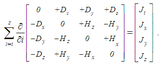 | (33) |
Regarding the incomplete symmetry, the trivial and dynamic (31b) equations form a similar tensor equation (34), with the opposite locations of the force fields, with respect to rational ones (33). Unlike the free term – in (33), expressing apparent electric, its absence in (34) points to the transparent magnetic carriers. The two tensors just concern the two distinct levels of the structure and consideration, electric or magnetic, mutually displaced along the structural depths. These two levels also accord with the rational or force fields – in the two tensors.
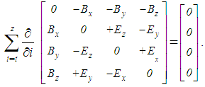 | (34) |
Apart from the field types – in the two field tensors, the opposite signs of the temporal terms accord with the opposite orders of the factors in Thomson’s relations, here transferred via Maxwell’s equations. This is finally manifest by the two opposite central forces, already interpreted by respective two temporal motions: of the particles – in the cosmic process, and their external kinetic flows. The formalistic CPT relation points to the symmetry of the circulations (in 3D sub-tensors) and the charge polarity – in the temporal and free terms, with respect to the steady course of time. 14
8. Energetic Balances
8.1. EM Field Energy
EM energy is expressed by respective force fields acting in the medium structure. The structural electricity, displaced from its regular position by electric forces, Fe = QE, obtains the potential energy (35). In a similar sense, magnetic forces acting on structural currents,  invest respective energy (36). The simple integration gives the expressions for respective two energy densities: We = ED/2 and Wm = BH/2. However, the integration of the former density in the space around a charge gives only a half of the energy obtained by radial integration of the central force.
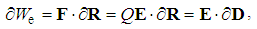 | (35) |
 | (36) |
As the mechanical analogy of this problem, let us observe a cylindrical spring stretched on an axial rod. The energy of the compressed rod must be added to this of stretched spring. The other question is do we use one or both energy halves at the spring realising. In the analogous way, the energy of the foreign fields must be added to the same density of that of the displaced electricity or current, as the two objects. The two equal and opposite internal force fields act from respective two structural strata. In the general sense, their balances point to the equal energy densities.
8.2. Continuity Equation
From the kinetic and dynamic Maxwell’s equations, a 5D continuity equation of EM energy can be obtained (37), just consisting of the spatial, temporal and substantial terms. Originally introduced accidentally, it is known as Poynting’s theorem. The first term represents the sources of the spatial energetic currents determined by the vector product of the two vacuum fields (38). Vector product of the two total fields is nothing else but, at least equivalent, mass current or linear momentum density.15 According to Maxwell’s relation (39), Einstein’s relation is finally obtained.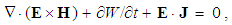 | (37) |
 | (38) |
The two famous relations are equivalent. As the typical speed of wave propagation, the former of them determines the speed of propagation by the elasticity and density of the medium (39), equal to the ratio of energy and mass currents. The medium rigidity, reciprocal to elasticity, is proportional to the energy current, but the medium density, including the vacuum and material strata, – to the mass current. Expressed in NS, these two currents at vacuum are mutually equal. At material media, with the slower wave propagation, mass is denser for the two material fractions.  | (39) |
The third term of (37),  represents the power of the ‘vertical’ energetic current, along the structural depths. It determines the transfer of EM energy into other forms. As the complement of spatial and structural flows, the second term determines the temporal variations of the same energy density in a spatial location and structural stratum. As such, it may be treated as the energy distribution along temporal axis. The continuity equation thus relates the three spatial and one temporal axis with the structural depth, as the fifth dimension. 5D space is thus finally completed. 16
9. Moving Entities
9.1. Structural Models
The convective derivative of the moving central field (3b) gives a toroidal vortex of displacement current, coaxial to the motion. It just continues the convection current of moving charge (Fig. 2). Including the circular magnetic field (11b), this is the photon associated to the moving particle. At the particle deceleration or full stoppage, it would be partially or fully liberated, continuing its free propagation at the speed c. The displacement currents are opposed by the strains of the medium structure, and so, the photon existence demands its own continuous axial propagation.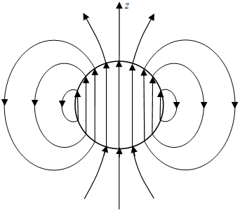 | Figure 2. Associated photon |
Unlike the convection current, collinear with the particle motion and respective kinetic potential (11a), the vortex of displacement current is only coaxial to the two mentioned vectors. Respective kinetic potential – in the same vortical form, is formed at the finer structure, and as such unmanifest on the material levels. Apart from above right screw photon, caused by the positive moving charge, the negative charge, with the opposite kinetic flows, is somehow predicted to produce the opposite, associated or free – left screw photon, similarly manifest in the experience.On the other hand, the hyper-toroidal kinetic potential (22), circulating in tr-planes and moving along temporal axis, may be nothing else but the particle model (Fig. 3). Really, the opposite circulation with respect to temporal axis forms the opposite charge polarity. Unlike axially symmetric photons, manifest by their magnetic fields and propagating through 3D space – as a moving frame, centrally symmetric particles, manifest by electric fields and respective masses, are moving into the future, thus determining the expanding cosmos itself, as the mentioned moving frame.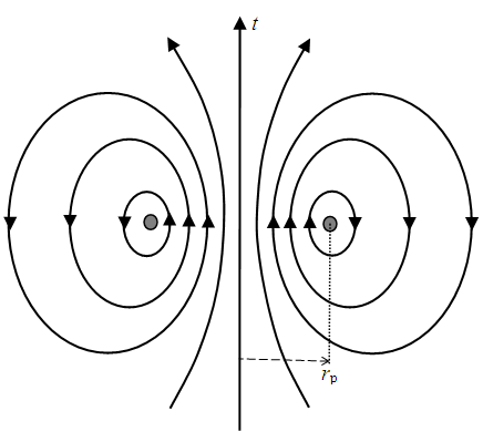 | Figure 3. Elementary particle |
The radial direction represents 3D space. The set of the centres of circulation in tr-planes forms the spherical surface in 3D. The kinetic flows diverge ahead, and converge behind a proton, as the positive particle, with the positive external, and negative internal potentials. (Fig. 4). All these facts are just opposite for an electron, as the negative particle. Thus obtained negative difference of the pressures on the proton surface determines the smaller radius and greater mass with respect to the same electron features. Of course, the particle mass is distributed in its external fields.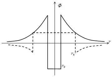 | Figure 4. Elementary potentials |
Apart from the compact vortices of photons and particles – propagating axially, the expanding alternating vortices – of EM waves – propagate radially. Unlike the photons, arisen at some deceleration and expansion of elementary particles, the waves arise from the oscillating processes, at collective flow of multiple particles in the technical generators. From a rod antenna the toroidal vortices are of the electric, with circular magnetic field. All is opposite from a loop antenna. In both these two cases, the wave polarization is determined by the electric field – in the antenna planes.
9.2. Motion Equations
Instead of Maxwell’s set and wave equation derived from it, let us present some applications of the algebraic relations to the treatment of EM waves, photons and charged particles. The substitution of Thomson’s relations (28), kinetic (a) into dynamic (b), gives the equation of motion (40a), and of (28a) – into Poynting’s relation (38) – gives the energetic current (41a). In various technical situations, at motion of the three mentioned entities, these equations are distinctly restricted. The two terms of each of these equations have the particular roles. Let us present the main cases. | (40) |
 | (41) |
In the case of both fields perpendicular to the motion, at waves or photons, the latter terms of these equations annul, reducing them into the former terms (b). The identity (40b) points to the distinct effective speeds of the two fields, with the known total speed, as their geometric average. Material media temporarily absorb respective fractions of the electric and/or magnetic energy, thus increasing its local density, and decreasing, in the same ratio, the speed of propagation. The remaining fraction of EM energy is propagating at the speed co, through the vacuum stratum only.The equality (41b) gives the effective current of energy. The energy density depends on the medium, but not on the particle speed. The moving energy can be increased by some expansion of the structural or spatial domains. The latter one is achieved by compression of moving particles. The latter term of (40a), with the longitudinal electric field, expresses the wave diffraction or expansion. The latter term of (41a) determines the opposite energetic flows ahead and behind the particle. The particle is borrowing some energy from, and returning the same power to the medium.
10. Summary
Introduction of Thomson’s algebraic relations was the first step of this elaboration. Comparison of the two fields around a moving charge obviously gave the kinetic relation, and the dynamic one was known as the empirical fact. The former of them relates the rational, and latter – force fields. At motion of one total, the other vacuum field is obtained. These two field relations announce their cyclic consideration. The two causal directions are distinguished by Maxwell’s equations. The trivial equation certainly excludes free magnetic poles and respective originating field.All the remaining Maxwell’s equations just emphasise the field hierarchy: from the static, via magnetic, to dynamic fields. The first field is originating, and two latter – vortical. These distinctions are additionally expressed by respective three elementary forces: radial – static, transverse – kinetic and longitudinal – dynamic. The static and dynamic forces are expressed by the collinear – electric, and kinetic one – by transverse magnetic fields. The additional algebraic relation (12b) determines the kinetic force, transverse to the magnetic field and motion of the object charge.The two fields in the algebraic pair, and their derivatives – in the differential set, point to the derivatives of the former, in order to obtain latter sets. However, the wider sense of the algebraic pair, for the spatial derivatives of the field speeds, was the problem in this procedure. It is surpassed by the fields understood as the rigid structures uniformly moving in space. Direct action at a distance of EM forces, without any temporal delays, is thus announced. The convective, directly give temporal derivatives, with a new restriction: the motion is effective only along the field gradient.The antinomy between the resting magnetic field and its motion with the carrying charge is resolved intuitively, by its transverse expansion and contraction. Respective speed field was primarily determined by the justifiable expectation of the zero torque acting on a moving electric dipole. The same function is convincingly interpreted as transverse convective derivative of the moving central potential. This confirmation just accords with the magnetic field lines understood as the isohypses of kinetic potential, with essential priority of EM potentials ahead respective fields.Full Maxwell’s set of the six equations clearly emphasises the hierarchy of EM quantities. Electricity and its current, as the apparent carriers, are the formal features of the fields, and the fields themselves – of respective potentials. This fact is manifest in the rational field tensor, with electric vortices in the longitudinal (tx, ty, tz), and magnetic – in the transverse (xy, yz, zx) planes of 4D space. The opposite locations of the force fields point to the electric and magnetic structural strata, or the levels of consideration. Instead of their 3D projections, the 4D originals are thus observed.The 5D continuity equation of EM energy determines its distribution in 5D space. Its three terms (spatial, temporal and substantial) represent the complementary motion and distribution of energy through 3D space, along temporal axis and structural depths of the medium. The law of neutrality, as the general form of the static equations, is also easily fitted into these frames. Moreover, the multiplication by length and division by time of the zero force sum points to the general energy homogeneity in 4D space. The opposite strains of the various strata compensate each other.The vortical particle model was formerly inspired by the same Descartes’ idea. Initially introduced very conditionally and checked carefully, it is gradually fitted into physical and formal relations during this elaboration. In the final instance, this theory and its further extension can be founded on this model [1]. With help of the two general laws, this model points to respective senses of gravitation and nuclear forces. This original approach to physics opens the door for the new direction of the scientific development. The majority of the speculative theories is thus bypassed.
11. Conclusions
In the gruelling inductive scientific development, each a step forward represents the scientific adventure. Therefore, unavoidable mistakes do not diminish the valuable results. Moreover, these results just enable the later correction of the mistakes. On the other hand, the great authorities of the same scientists, deserved by their results, also prevent their own mistakes from the scientific critique. The little initial errors thus grow and multiply in time, up to untenable deviations. By this logic, the erratic essences of the modern speculative theories may be expected. In this systematic exposition of EM theory, a sequence of the former mistakes is pointed at and substituted by the more consistent and convincing alternatives. Such examples are Ampere’s failure to formulate the general kinetic law and Maxwell’s successive transfer of physical forces. Via Hertz’ symmetry of Maxwell’s equations and Dirac’s prediction of magnetic monopoles, these initial errors culminated into the special relativity, quark and string theories, elementary mass, and so on. The initial rational bases degenerated by the time into scientific speculation or fiction.From the further infinite development or maintenance of this speculative creation, its uncontrolled collapse would be worse. Its partial reconstructions threaten with such an effect. Therefore, scientists are very intolerant of essential critique of the main scientific orientation. Instead of such risky tries, the reliable fundaments of physics are to be separated aside, enabling two or more parallel competing developments. The elaborate EM theory, as the central physical discipline, might be such an alternative basis. Apart from mechanics, it also refers to microstructure and cosmology.
Notes
1. The medium is a substantial content of the formal frame.2. Instead of elasticity, the inverse rigidity is usually used.3. The form of equations is disturbed in some obsolete systems.4. Owing to inertial and gyroscopic effects of EM fields, free or associated to the carriers, they usually move uniformly.5. Of course, the moving negative static, would form the opposite kinetic quantities, in the given formal frame.6. With respect to (2), the sequence (12) is also consistent.7. The cosmic process is neither accelerated nor decelerated – but uniform, determining the continual lapse of time.8. Unlike the similar external fields of electric and magnetic dipoles, respective two internal fluxes are opposite.9. Apart from the general dependence on the mutual position, these two forces also depend on the speed products. 10. Without strict argumentation, the field deformation is predicted by H. A. Lorentz, but 2/3 of the elementary charge is needed in the quark theory, concerning the speedy particles.11. Amongst the charge particles, as the apparent field carriers, there is no any place for the assumed mass bosons.12. With respect to all the three EM forces already understood in the former transformation, this one is excessive. 13. All aspects of this conception are extremely problematic.14. This symmetry, interpreted in the note 5, is also extended to the time inversion – in the complete Maxwell’s set.15. Unaffected by the usual forces, this mass and linear momentum are manifest by the wave pressure on irradiated surfaces.16. One leg of this axis strives into structural depths, and the other – into cosmic widths, both without known limitations.
References
| [1] | B. Mišković, Reexamination of Physics, in preparation. |
| [2] | B. Mišković, Fundamentals of Electrodynamics, SAP, I. J. of Electromagnetics and Applications, 5(1), 2015. |
| [3] | B. Mišković, Space, Time and Motion, SAP, I. J. of Theoretical and Mathematical Physics, 5(2), 2015. |
| [4] | B. Mišković, Final Essence of Material Existence, SAP, I. J. of Theoretical and Mathematical Physics 5(1), 2015. |
| [5] | B. Mišković, Relativity and/or Symmetry, SAP, I. J. of Theoretical and Mathematical Physics, 4(5), 2014. |
| [6] | B. Mišković, Medium of Natural Phenomena, SAP, I. J. of Theoretical and Mathematical Physics, 4(4), 2014. |

 Abstract
 Reference
 Full-Text PDF
 Full-text HTML