Estomih S. Massawe
Department of Mathematics, University of Dar es Salaam, Dar es Salaam, Tanzania
Correspondence to: Estomih S. Massawe, Department of Mathematics, University of Dar es Salaam, Dar es Salaam, Tanzania.
| Email: |  |
Copyright © 2016 Scientific & Academic Publishing. All Rights Reserved.
This work is licensed under the Creative Commons Attribution International License (CC BY).
http://creativecommons.org/licenses/by/4.0/

Abstract
In this paper it is intended to elaborate a framework in which we can incorporate external forces in the systems prescription with emphasis on Hamiltonian systems with external forces and on the consequences of external forces. An appealing tool for this case is the language of symplectic geometry. Definitions of Hamiltonian systems with external forces are given and it is shown how they fit very naturally into the framework. It is also shown that forces are basic variables and that they have to be included in the definitions of mechanical systems.
Keywords:
Hamiltonian, Control systems, Controllability, Observability
Cite this paper: Estomih S. Massawe, Hamiltonian Control Systems, International Journal of Theoretical and Mathematical Physics, Vol. 6 No. 1, 2016, pp. 26-30. doi: 10.5923/j.ijtmp.20160601.02.
1. Introduction
The dynamics of a system can be formulated using either the Newtonian, the Lagrangian or the Hamiltonian approaches. In the Newtonian and the Lagrangian formulations it is assumed that if all the coordinates and velocities are simultaneously specified, the state of the system can be completely determined and its consequent motion calculated. This gives rise to solving a system of second order ordinary differential equations. On the other hand, the Hamiltonian formulation, we seek to describe the motion in terms of first order equations of motion parametized by generalized coordinates and momenta. The transition from the Newtonian and Lagrangian formulations to the Hamiltonian formulation corresponds to changing the variables in the system from  to
to  where
where  are the generalized coordinates and
  are the generalized momenta [1]. However the Hamiltonian methods are not superior to the other methods for direct solutions of mechanical problems. Rather we gain another more powerful method of working with physical systems. The usefulness of the Hamiltonian viewpoint lies in providing a framework for theoretical extension in many areas of physics such as statistical mechanics and quantum mechanics.A Hamiltonian system is characterized by an existence of a symplectic structure on a smooth even-dimensional manifold [2]. The symplectic approach allows one to extend the local description of a dynamical system to a global description. [3] has shown how network modelling of lumped-parameter physical systems naturally leads to a geometrically defined class of systems, called port-controlled Hamiltonian systems with dissipation. The structural properties of these systems were discussed, in particular the existence of Casimir functions and their implications for stability. [4] has shown the geometric property and structure of the Hamilton--Jacobi equation arising from nonlinear control theory are investigated using symplectic geometry. [5] made an analysis on Hamiltonian systems and his results revealed a systematic geometric frame for generalized controlled Hamiltonian systems. The pseudo-Poisson manifold and the ω-manifold are proposed as the state space of the generalized controlled Hamiltonian systems were established. However the above results did not consider the external forces as basic variables.In this paper it is therefore intended to show that external forces should. It will be shown that it is necessary to maintain forces as basic variables and those have to be included in the definition of mechanical systems.
2. Hamilton’s Equation
Let  be the Lagrangian function for a given system. Then the Hamiltonian function
  for the system is defined by ([1], [6]).
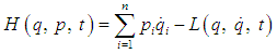 | (1) |
The differential of  is given by
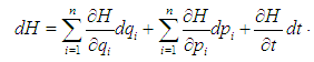 | (2) |
Also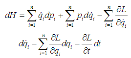 | (3) |
Using  from the generalized momenta, equation (3) reduces to
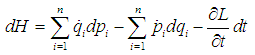 | (4) |
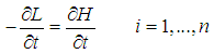
Comparing (4) and (2) we get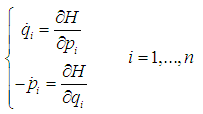 | (5) |
 | (6) |
Equations (5) consist of a set of  first order ordinary differential equations called the Hamilton’s equations of motion and
  are called canonical coordinates.
2.1. Hamiltonian Control Systems
According to [2] we let●  be a manifold
  of the state space in a manifold with symplectic form
  ,●
,●  be a manifold of the space of external variables with symplectic form
  (‘e’ for external). In local coordinates,
  where
where  are the external forces (inputs) and
  are the observations (outputs),● A fiber bunder
  be over
  ,● A smooth function (smooth meaning
  ) such that
  (
( is a tangent bundle over
  .Then(i)
  with
with  and
and  symplectic manifolds is called a full Hamiltonian system if
  is a Lagrangian submanifold of
  where
where 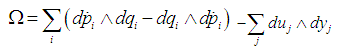 is derived from the local coordinates.(ii)
  is called degenerate Hamiltonian system if there exists a full Hamiltonian system
  such that
  is a submanifold of
  .The definition of Hamiltonian control system depends on the submanifold
  and not on
  and
and  separately. It can be observed that the set of external variables
  can be split into inputs
  and outputs
  . The inputs are the external forces (controls) and the outputs are the observations. If the external forces are constant, then the dynamics of the system are described by a Hamiltonian vector field on
  .
.
2.2. Affine Hamiltonian Control Systems
Let  be a symplectic manifold. Let
  be an observation manifold. Define the symplectic form
  on
on  by
by  (
( is the cotangent bundle of
  ,
,  and
and  are pullbacks of
  and
and  by
by  and
and  respectively [2]. Then according to [7] an affine Hamiltonian system
  is given by a submanifold
  such that(i)
  can be parametized by the coordinates of
  and the coordinates of the fibres of
  ,(ii)
,(ii)  is a Lagrangian submanifold of
  ,(iii) The value of the
  -coordinates of a point on
  is a function only of the
  -coordinates of this point.This system is thus given by ([8])
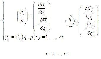 | (7) |
In vector form we denote the system (7) by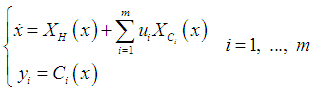 | (8) |
Because of (ii) above,  has a generating function. Because of (i) and (ii), this generating function has then form
 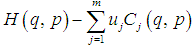 with
with  canonical coordinates for
  and
and  natural coordinates for
  . Therefore
  coordinates of
  are given by
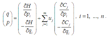 | (9) |
and the  coordinates by
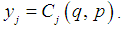 This is equivalent to linearizing
  with respect to
  . We note that without condition (iii), the external forces enter the system in a nonlinear way and the generating function of
  is
is  which locally gives
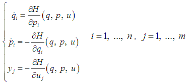 | (10) |
This is just the usual general input-output Hamiltonian system. We note that if there are no dynamics i.e. no state space  , then
  is just a Lagrangian manifold of
  and this describes statistic mechanical systems. If there are no inputs and outputs i.e. no
  , then
  is a Lagrangian submanifold of
  . This describes a locally Hamiltonian vector field.
2.3. Linear Hamiltonian Control Systems
The Linear system in state form 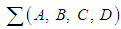 given by
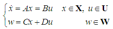 | (11) |
is a linear Hamiltonian system if  and
and  are symplectic linear spaces. It is a result in symplectic geometry that there exists a nondegenerate skew-symmetric bilinear form
  and
and  on the state space
  and on the set of external variables
  respectively ([2]). In the same language o symplectic geometry if
  and
and  then there exists bases of
  and
and  such that in these bases
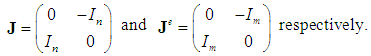 [9] has established and proved by the following theorem the conditions required for the system
  above to be a full linear Hamiltonian system.Theorem 1:Let
  be a linear system given by (11) above. If
  is injective and
  are linear symplectic spaces, then
  is a full Hamiltonian system if
  and
and  satisfy the following:
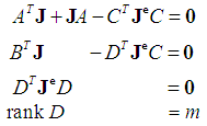 | (11) |
If the feedback given by 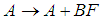 ,
, 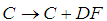 is applied to
  , then necessarily
 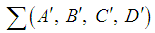 has to satisfy
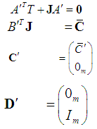 | (12) |
where The condition that
  is injective is similar to the condition that
 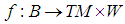 is an embedding for the case of nonlinear systems.
3. Controllability and Observability for Hamiltonian Systems
We shall consider the ideas of controllability and observability only for affine nonlinear Hamiltonian systems. Consider the system given by 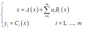 | (13) |
Defined on a symplectic manifold  where
where  is a locally Hamiltonian vector field i.e. the Lie derivative
  . And
. And  is the Hamiltonian vector fields such that
  ([10]).Definition 1Consider the affine system (13) above. We define
  and
and  . This system is locally weakly observable if
  satisfies
  Here
Here  is the linear subspace of
  spanned by
  with
with  [11].For Hamiltonian systems, since
  and there exists
  such that
  then the
  defined above satisfy
  with
with  the affine subspace of vector space of functions on
  . ([6])We define Controllability and Observability as follows:Controllability: Controllability is the set of points reachable from
  in time
  by applying input functions
 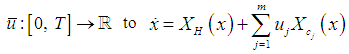 with initial condition
  contains an open subset of
  for every
  and for every ([9]).Observability: For every
  and every
  there exists a neighbourhood
  of
of  such that for
  and
and  in
in  and
and  , there exists input functions
  such that, if we denote the solutions of
 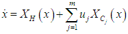 on
on  corresponds to initial conditions
  and
and  by
by  and
and  respectively, then the output functions
  and
and  are different while the trajectories
  and
and  remain in
  ([9]).
4. Feedback for Hamiltonian Systems
Define a function  such that
  , where
  is a closed one-form on the output
  , and consider the output feedback given by
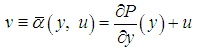 | (14) |
Let  be the graph of
  and
and  be a Lagrangian submanifold i.e.
  . Accordingly we say that the output feedback given by equation (14) is Hamiltonian ([5]).Proposition 1Let
  be an affine Hamiltonian system given by
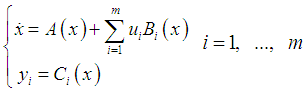 with
with  and so
  and
and  i.e.
i.e.  ([5]). Let
  be a feedback for this system. After feedback, this system will again be an affine Hamiltonian system.
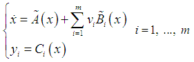 iff
iff  is a Hamiltonian feedback i.e. there exists a function
  such that
  and
and  satisfy
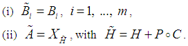 Hence Hamiltonian feedback adds a potential function which is only a function of the output.Let us now consider a solution of Disturbance decoupling by observation feedback (DDOF). The formulation of DDOF is as follows: Let
 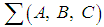 be a Hamiltonian system on a symplectic space
  where
where  . It is assumed that there are disturbances in this system and it is intended to control the state space. The system can be described by
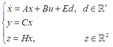 with
with  the disturbances and
  the variables which are to be regulated. We shall call
 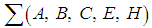 with
with 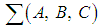 Hamiltonian and
  a Hamiltonian system with disturbances. Then the DDOF problem is to find a compensator
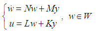 Such that the closed-loop system
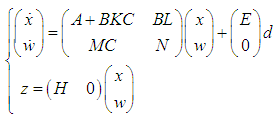 decouples the disturbances
  from
from  .We shall require
  to posses a symplectic form
  and
and 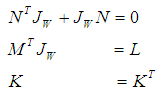 Proposition 2Let
  be a Hamiltonian system with disturbances. Then(i) DDOF is solvable iff there exists an
  -invariant subspace
  contained in
  and which is coisotropic ([10]).(ii) DDOF is solvable if the pullback
  is coisotropic ([7]).Let
  be a Hamiltonian system with disturbances. Let
  be
be  -invariant and Lagrangian, so DDOF is solvable by static output feedback
  . Then also the Hamiltonian output feedback
  solves DDOF. ([7]).
5. Discussions and Conclusions
In the past, most treatments in classical mechanics have dealt only with analytical mechanics. This part of mechanics confines itself to the study of mechanical systems without external influences. When forces are present they are assumed as coming from a potential field. In this context one observes the motions, makes classifications etc. i.e. one does only descriptive work but cannot influence the behaviour of the system. This restriction entails a heavy loss of generality because external forces do come up at various places for instance experimental devices and technical applications and mostly cannot be derived from a potential function. Control theory on the other hand does prescriptive work. One attempts to express all models in input/output form so that the variables which may be manipulated and observed are clearly distinguished. Also one tries to find methods for regulating the response of systems by altering the equations of motion. Problems of this type are very natural i.e. in engineering, operational research, and in economics where the problems are laid out in terms of the decision variable (inputs) which have to be chosen on the basis of certain observations (outputs) and the mathematical model involves the interrelations between these variables. The Newtonian and Lagrangian approaches are as good as any other but it is more advantageous to develop the Hamiltonian point of view because it reveals certain structural features e.g. we can anlyze the non-linear systems globally; conservation laws follow easily. In this paper, a framework in which we can incorporate external forces in the systems prescription with emphasis on Hamiltonian systems with external forces and on the consequences of external forces has been elaborated.
References
| [1] | H. Goldestein, Classical Mechanics, Addison-Wesley, Reading, Massachusettes, 1980. |
| [2] | R. A. Abraham, J. E, T. Ratiu, Manifold Tensor Analysis and Applications, 2nd edition, Springer-Verlag, New York, 1988. |
| [3] | A. van der Schaft, Port-controlled Hamiltonian systems: towards a theory for control and design of nonlinear physical systems, Journal of the Society of Instrument and Control Engineers of Japan (SICE), Vol. 39, nr. 2, pp. 91- 98, 2000. |
| [4] | N. Sakomoto, Analysis of the Hamilton--Jacobi Equation in Nonlinear Control Theory by Symplectic Geometry, SIAM Journal on Control and Optimization, Volume 40 Issue 6, 2001, p. 1924 – 1937. |
| [5] | D. Cheng, Z. Xi, Q. Lu, Sh. Mei, Geometric structure of generalized controlled Hamiltonian systems and its application, Science in China Series E: Technological Science, August 2000, Volume 43, Issue 4, p. 365-379. |
| [6] | L. P. Landau and E. M., Lifschitz, Mechanics, Pergamon Press, Oxford, 1976. |
| [7] | A. J., Van der Schaft, “System Theoretic Properties of Hamiltonian Systems with External Forces”, Dynamical Systems and Microphysics Control Theory and Mecanics, pp. 379-399, Academic Press, 1984. |
| [8] | A. J. Van der Schaft, Hamiltonian Dynamics with with External Forces and Observations, Mathematical Systems, SIAM Journal of Control and Optiization, Vol 20, pp. 338-354, 1982. |
| [9] | R. Herman and A.J. Krener, “Nonlinear Controllability and Obervability”, IEEE Trans. Automatic Control, Vol. AC-22, pp. 728-740, 1977. |
| [10] | A. J. Van der Schaft, Disturbances Decoupling by Observation Feedback for Hamiltonian Systems, System and Control Letters,, Vol. 2, pp. 286-291, 1983. |

 Abstract
 Reference
 Full-Text PDF
 Full-text HTML