Bratianu Daniel
Str. Teiului Nr. 16, Ploiesti, Romania
Correspondence to: Bratianu Daniel, Str. Teiului Nr. 16, Ploiesti, Romania.
| Email: |  |
Copyright © 2015 Scientific & Academic Publishing. All Rights Reserved.
This work is licensed under the Creative Commons Attribution International License (CC BY).
http://creativecommons.org/licenses/by/4.0/

Abstract
This paper tries to prove that the existence and properties of the electron’s spin can be established not only as a consequence of relativistic quantum mechanics, but also as a consequence of non-relativistic quantum mechanics of the Hydrogen atom or Hydrogenic atoms. It is, in fact, an extended model of the Hydrogen atom or Hydrogenic atoms. This new model starts from the assumption that to the foundation of atomic structure there is not only a potential of electrical nature, but also a potential of magnetic nature, which, together with the Coulomb potential, determine the movement of electrons around the atomic nucleus. As a consequence of this new model is obtained a non-relativistic theory of Hydrogen atom which takes into account the spin of the electron and leads us to a non-relativistic theory of the atom in agreement with the Stern-Gerlach experiment results. As well the model can be used in order to explain the spectrum of Alkali-atoms.
Keywords:
Spin, Magnetic field, Virtual, Nonrelativist, New model, Extended
Cite this paper: Bratianu Daniel, The Hydrogen Atom – Extended Model, International Journal of Theoretical and Mathematical Physics, Vol. 5 No. 6, 2015, pp. 151-159. doi: 10.5923/j.ijtmp.20150506.01.
1. Contents
Let us consider an electron that moves with velocity  on a circular orbit in the meridian plane of a nucleus.Such an electron produces a "current loop" in this plane. From the fundamental laws of electromagnetism we know that any current loop produces a magnetic field perpendicular oriented to the plane of the orbit. The expression of the magnetic field at the center of such a "current loop" can be described, according to the laws of electromagnetism, by the formula:
 | (1) |
where  is the vacuum magnetic permeability,
  is the radius of the current loop, and
  is the circulating current . Further, instead of using Cartesian coordinates
  , it is convenient to introduce spherical coordinates
  :
: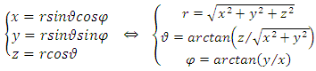 | (2) |
Therefore, we can assume that the component of the magnetic induction in the  direction is
  because
  is the radius of the current loop in the meridian plane. But, from the electron’s point of view, the nucleus revolves around him. Thus, the nucleus produces also a “current loop”. Therefore we can assume that the expression of the magnetic induction
  of the magnetic field produced by nucleus in the point where is placed the electron, has the form
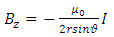 | (3) |
(the minus sign appears because the two systems, electron and atomic nucleus, have the opposite velocities,  and
and  ). Now, as expression of circulating current
  we can introduce the formula
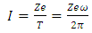 | (4) |
where  is the elementary charge,
  is the atomic number, and
  is the orbital period of the atomic nucleus. For the angular velocity of the nucleus
  we allow the formula
 | (5) |
where  is the phase velocity of the de Broglie wave associated with the atomic nucleus. Thus, the expression of the circulating current
  of the atomic nucleus becomes
 | (6) |
Substituting this expression in the expression of magnetic induction  , we get
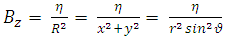 | (7) |
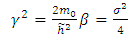
where the constant  is given by
 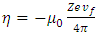 | (8) |
Further, we introduce the formula  , where
  is the speed of light and
  is the vacuum permittivity, so that the constant
  of
of  (8) can be rewritten as
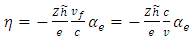 | (9) |
where  is the fine structure constant,
  is the reduced Planck constant, and
  is the well-known expression
  . Thus, we admit that from the electron’s point of view, the nucleus produces a magnetic field, whose expression can be written in vectorial form as
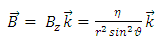 | (10) |
where  is the unit vector along
  axis, and
  is the
  component of the magnetic induction
  . Therefore, in order to correctly describe the motion of the electron, we must appeal to the Hamilton function of a particle with electric charge
  , located in an electromagnetic field represented in terms of the scalar and vector potentials
  and
and  . So, we introduce the Hamiltonian operator of the form
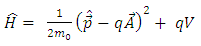 | (11) |
where | (12) |
is the expression of the scalar potential  and
and  is the rest mass of the electron. We do not know the expression of the vector potential
  . But, we know that for an electron located into a constant magnetic field, we can write this expression as
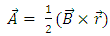 | (13) |
We keep this expression for the case when the magnetic induction ( ) is a function of the position
  of the electron. Therefore, substituting
  (10) into
  (13), the vector potential
  becomes
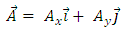 | (14) |
where  and
and  are
are  and
and  components of the potential vector
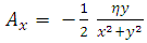 | (15) |
 | (16) |
in Cartesian coordinates  , and
, and  . Now, if we apply the transformations (2), we get
 | (17) |
 | (18) |
in spherical polar coordinates  . Thus, the Hamiltonian operator
  of the electron can be decomposed as the sum
 | (19) |
where the expressions of the operators  and
and  , according to
  (11), are given by the formulas
 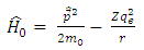 | (20) |
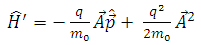 | (21) |
Now, with the aid of components  and
and  and of the transformations (2), we can find the expressions
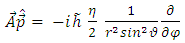 | (22) |
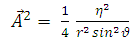 | (23) |
so that  can be written as
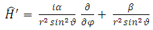 | (24) |
where the constants  and
and  are given by the relations :
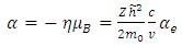 | (25) |
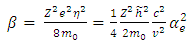 | (26) |
in which  is the Bohr magneton
 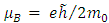 . Let us now consider the Schrodinger equation for an electron in the electromagnetic field of a nucleus of charge
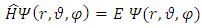 | (27) |
We assume a variables separable solution to this equation of the form 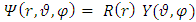 . Substituting this solution in
  (27), after the separation of variables, we get the following two independent equations:
 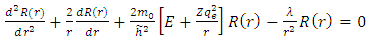 | (28) |
for radial wave function, and respectively 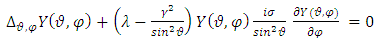 | (29) |
for the angular wave function, and the constants are given by the formulas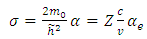 | (30) |
 | (31) |
 | (32) |
The constant  is the separation constant, and
 signifies the angular momentum squared. We assume again a variables separable solution to the second equation
  (29) of the form
 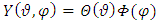 . Thus this equation can be separated in others two independent equations
 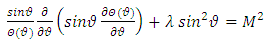 | (33) |
and respectively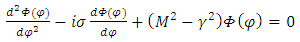 | (34) |
where the constant  is the separation constant. After the change of variable
 , the first equation
  (33) can be rewritten as the well-known equation
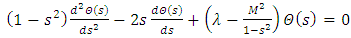 | (35) |
For the second equation  (34), we assume a solution of the form
 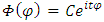 , where
  is a real constant. From the normalization condition we find the value of constant
  as
as  . Inserting the solution of
  into Eq. (34), we obtain now the following characteristic equation
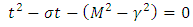 | (36) |
This is a quadratic equation for which, according to Eq. (31), we find the roots | (37) |
Now, we must consider the azimuth boundary condition  which imposes the conditions
  | (38) |
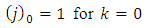
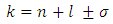
where  is a positive integer (including zero). Thus, we can write the constant
  as
as  , where we have used the notation
  . Further, we introduce for the constant
  another notation
  , so that we can write
 | (39) |
where  is the well-known orbital magnetic quantum number. Therefore, the solution
  becomes
  | (40) |
Turning now to  (35), we assume here a solution of the form
 | (41) |
which replaced in this equation leads us to the following differential equation for unknown function 
 | (42) |
In order to exclude the singularities of the points  , we must impose the condition
  which generates the values of the exponent
  as
as | (43) |
and the equation  (42) gets the following well-known form
 | (44) |
A solution may be found if we admit for  the value
  . With this value for
  , the solution
  of Eq. (44) can be written as
 | (45) |
if we admit that the constant  has the expression
 | (46) |
where  | (47) |
 | (48) |
(the proof of formulas (46), (47) is provided by the Annex 1)Another solution for  may be also
 | (49) |
for the same  and
and 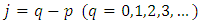 Indeed, if we substitute
  in Eq. (30) and Eq. (39), we find that the velocity of the electron
  gets the expression
  | (50) |
and the quantum number  becomes
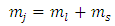 | (51) |
where  is the spin magnetic quantum number
  From Eq. (43) and Eq. (47), we can obtain now the formula
  | (52) |
where  is the orbital quantum number, given by the formula
 | (53) |
Also, from Eqs. (43) and (47), we can find the inequalities | (54) |
where  and
and  take only half-integers values (It should be mentioned here that in the state
  the quantum number
  can have a single value,
  , so we can write
  ). Substituting now the solution
  of Eq. (45) into Eq. (41), for
  , we can write the solution
  of Eq. (35) in the general form
 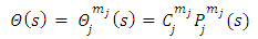 | (55) |
where the  function is the solution Legendre's equation Eq. (35) for the half-integers quantum numbers
  and
and 
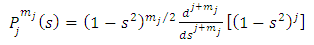 | (56) |
Because this solution must be finite on the interval  we must permit for
  only the values
  . The constants
  are the multiplication factors determined by the normalization condition which gives
 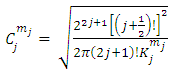 | (57) |
(the proof is provided by the Annex 2)The expression of the  coefficients is given by the formula
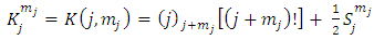 | (58) |
the coefficients  have the expression
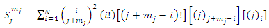 | (59) |
and the symbols  are given by the expressions
 | (60) |
 | (61) |
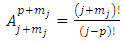
The  upper limit of the sum from Eq. (59) is
 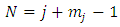 and the symbols
  are combinations of
  from a set of
  (the binomial coefficients).
 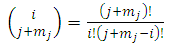 | (62) |
Now, it is convenient to define a radial coordinate with no units as  where
where  is the unit length or radius of the first Bohr orbit
 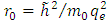 . Thus, we obtain the radial equation Eq. (28) for the Hydrogenic atom as
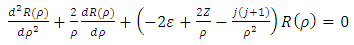 | (63) |
where ε is a dimensionless constant 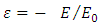 and
and  is known as the energy unit. We assumed now a solution of the form
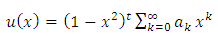
 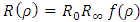 to this equation, where we have
  and
and 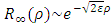 as asymptotic solutions of radial equation. Further, for generality, we can write
  | (64) |
Substituting the solution  into radial equation Eq. (63), we find the equation for the unknown radial function
 | (65) |
where we have introduced the notation  . We can simplify this equation if we introduce a new variable with no units
 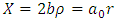 where
where  so that we can write our differential equation as
  | (66) |
Now we can make the notations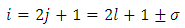 | (67) |
 | (68) |
 | (69) |
where the indexes  and
and  must be integers. So we can bring the equation to the following final form
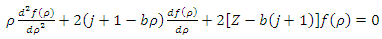
 | (70) |
The solution of this equation is a polynomial of degree 
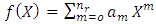 which leads us to following recursion relation between coefficients
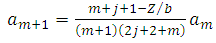 | (71) |
Because the maximum value of  is the degree of the polynomial, we find the condition
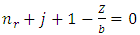 | (72) |
Therefore, the polynomial  is the same well-known generalized (associated) Laguerre polynomial
  . So, the radial wave function
  may be written as follows
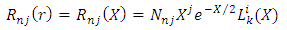 | (73) |
where  are the multiplication factors, whose expression can be determined by the normalization condition of the wave function
 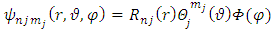 which leads us to the following equation
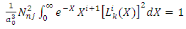 | (74) |
Using here the orthogonality condition of Laguerre polynomials written as 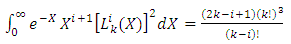 | (75) |
the normalization condition Eq. (74) takes the form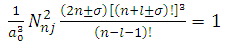 | (76) |
from which we deduce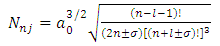 | (77) |
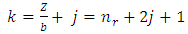
Substituting now Eq. (64) into Eqs. (72) and (70), taking into consideration the expression of principal quantum number 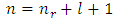 , we get the formulas
 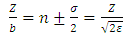 | (78) |
 | (79) |
Therefore, we find that the total energy eigenvalues for the Hydrogenic atom are given by the expression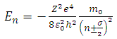 | (80) |
2. Conclusions
A first conclusion that can be drawn from this extended model of the hydrogenic atom is that the changes produced by the own magnetic field  in the evolution of this type of atom are taken into account through the dimensionless variable
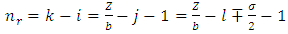
  . From the above definitions of the indices
  and
and  , in which this variable plays an important role, we deduce that it must be an integer. Also, we can observe that there is a relationship between the variable
  and velocity of the electron
  , according to the formula Eq. (30). From this formula we can deduce that the number
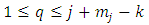
  must be positive. Also, from the condition
  , we get
 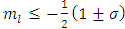 . As well, from Eq. (53), we can find the inequality
  . Further, from these inequalities we get the condition
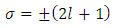 | (1) |
Therefore, we can consider that the  variable is an positive integer
  . So, we can observe that for
  odd, although the electron spin stands out, the total energy formula does not correspond to the experimental results. This weakness of the model is certainly due to the fact that he does not take into account the radiative reaction force (the self force) which acts on the electron. Howbeit, if we admit that
  and we rewrite the radial equation Eq. (28) as follows
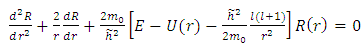 | (2) |
we can observe that it is possible to introduce here another expression for the potential energy  of the atom, as
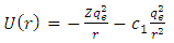 | (3) |
where  is a positive constant
  . Indeed, taking into consideration the expressions of the quantum numbers,
  and
and  from Eqs. (46) and (64), we obtain the equation
 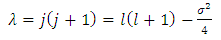 | (4) |
where we have chosen  . Therefore, we can identify the second term of this equation as
 | (5) |
From this equation we can introduce the physics quantity  | (6) |
which is named the quantum defect, and for which the experimental formula can be given by the following expression | (7) |
where  is a positive constant, too. These formulas are the experimental formulas of the alkali atoms. For these atoms the energy eigenvalues are in accordance with the expression Eq. (80), for
  . Also, it can be shown that if we take
  , and we introduce the formulas
  ,
,  ,
,  , can be obtained a theoretical situation in agreement with the results of the Stern-Gerlach experiment. The expression of the electron energy eigenvalues, for
  , can be written as
 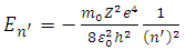 | (8) |
where  becomes principal quantum number.
ANNEX 1
Let us consider the equation for  function
 where
where  . We can look for the solution as a product between the function
  , raised to a power
  , and a power series in
 | (2) |
Substituting this solution into the initial equation Eq. (1), we get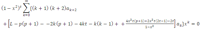 | (3) |
This equation has the singular points  . In order to exclude them, we rewrite the numerator of the fraction as
 | (4) |
Now we can obtain a simplification of the fraction if we impose the condition  . Therefore, we get for the power
  the values
 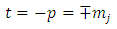 | (5) |
and the initial ecuation Eq. (1) becomes | (6) |
Now, after a rearrangement of terms, we rewrite this equation as | (7) |
which leads us to the following recursion relation between the coefficients 
 | (8) |
We impose now the condition as the series be reduced to a polynomial of maximum degree 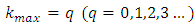 . Therefore, the recurrence relation Eq. (8) leads us to the formula
 which can be written as
 | (9) |
where | (10) |
QED.
ANNEX 2
Starting from the solution of the Legendre equation for half-integers numbers 
 | (1) |
where the function  has the expression
  and is defined over the range
  , we can show the orthogonality of
  functions with the same superscript
  , but different subscripts
  and
and 
 | (2) |
Also, we can calculate the expression for the coefficients of normalization  , when the indices
  and
and  are half-integers numbers. Substituting the solutions Eq. (1) in the integral Eq. (3), we get
 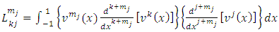 | (3) |
from which we can see that the indexes  and
and  occur symmetrically and, therefore, without loss of generality, it is enough to investigate the case
  . We use now the formula of integration by parts
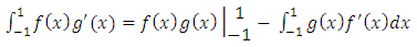 | (4) |
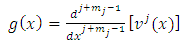
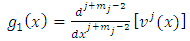
where, we note by  the first bracket, and by
  the two
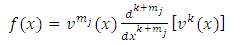 | (5) |
 | (6) |
After the first integration, we obtain the following expression for 
 | (7) |
We continue the integration by parts, making the notations 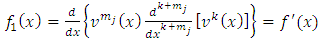 | (8) |
 | (9) |
Applying again the formula of integration by parts Eq. (4), we obtain  | (10) |
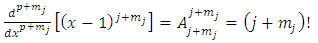
Taking the  derivative of
  , we obtain
 | (11) |
Now we can see that 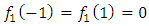 if
if  , so the integrated term will be zero, because it contains the
  factor to a minimum power,
  (where number 2 indicates the number of integrations), and the same
  factor to a maximum power,
  , and therefore, this factor will be zero at both endpoints
  . Continuing the integration by parts, we can see that the degree of the derivative of the
  increases by 1 on each integration, while the degree of the derivative of the
  is reduced by 1 on each integration. After a number of
  integrations by parts, the
  factor of the integrated term will be composed from a sum of terms which will include the
  factor at the half-integers powers which extend from
  to
to  . All these terms will be zero at both endpoints, if
  . So, after a number of
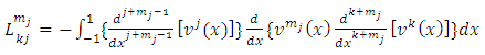
  integrations by parts we can write the expression of
  Eq. (7) as follows
 | (12) |
where | (13) |
 | (14) |
As we have seen above, for  , the
, the  factor of integrated term will be zero. For
  , this factor will no longer be zero. However, this time will be zero the second factor of product,
  , because, after we calculate higher and higher derivatives, we will have a sum of terms containing the
  function as factor, and the lowest power of
  in any of these terms will be
  so that every term will go to zero at the endpoints. Therefore, if we integrate by parts
  times, we get
 | (15) |
Now if we let  , since
  and
and  appeared symmetrically in the initial integral, we may write
 | (16) |
Also, we may consider the case  , which covers all possible cases. Further we can write the
  function as follows
 | (17) |
Using the higher derivative formula for the product (the Leibniz’s rule), we take the  derivative of this function of the form
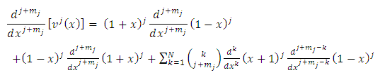 | (18) |
where 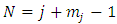 . Since each derivative of the function
  brings down the exponent and then reduces the exponent by 1, we may write
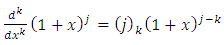 | (19) |
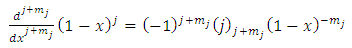
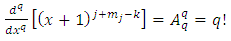
or correspondingly for the function  , we may also write
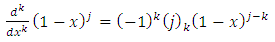 | (20) |
Now if we let  into Eqs. (21) and (22), we obtain
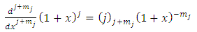 | (21) |
 | (22) |
or, using the same symbol, we may also write 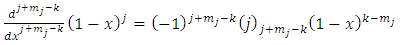 | (23) |
If we replace these formulas in Eq. (18) and then we multiply both sides of equation by the functions  , we obtain
 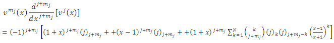 | (24) |
Now taking the  derivative of this expression, we get
 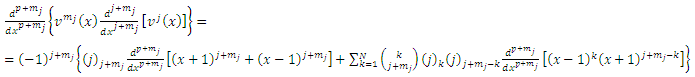 | (25) |
Since the indexes  and
and  are half-integers numbers, the numbers
  and
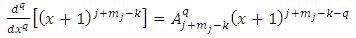
and  will be integers . Therefore, we can introduce the following higher derivatives formulas
 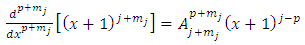 | (26) |
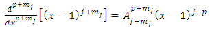 | (27) |
where the symbols  are the permutations of
  from a set of
 | (28) |
where we must impose the inequality  . Also, we can use now the inequality
  . Adding the
  in the both members of this inequality, we get
  . From these inequalities we find the condition
  . Applying again the Leibniz's rule, further we may write
  | (29) |
where 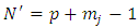 . Since
  , the index
  is an integer in the range
 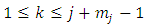 . Therefore, the first two terms of this equation will be zero. So, we can write
  | (30) |
Now we use again the higher derivatives formulas as follows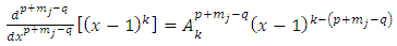 | (31) |
 | (32) |
where we must impose the inequalities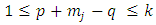 | (33) |
 | (34) |
from which we deduce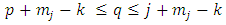 | (35) |
So, we have for the two indexes,  and
and  , the conditions
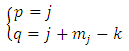 | (36) |
Inserting these conditions in Eqs. (31), (32) we get 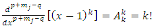 | (37) |
 | (38) |
Also, we get 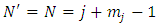 . Therefore, the expression Eq. (30) takes the final form
 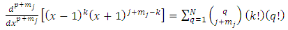 | (39) |
This is different from zero only when  . For
. For  will be zero. Also, for
  , Eqs. (26) and (27) becomes
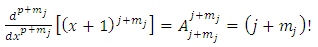 | (40) |
 | (41) |
Thus, for  ,
,  (25) can be written as
  | (42) |
where, if we replace  and we take into consideration the relations
 | (43) |
we can write this equation as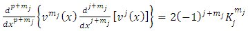 | (44) |
Therefore, the integral  Eq. (16) takes the following form
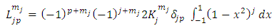 | (45) |
where, in agreement with the previous results, we have used here the Kronecker symbol  that shows the orthogonality of functions
  with
with  . Thus, for
  , the integral
  (45) becomes
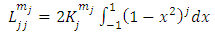 | (46) |
The final integral can be evaluated by using the trigonometric substitution  and the trigonometric formula
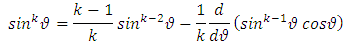 After an integration by parts, the integral can be written as
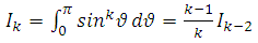 | (47) |
where  . Therefore, we can establish the following formula
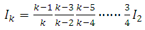 | (48) |
Since  is an even number, we can write
 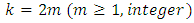 and the integral
  (48) becomes
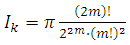 | (49) |
or, using the quantum number  , the integral gets the formula
 | (50) |
So, plugging this back into Eq. (46), we get finally | (51) |
Now if we write the normalization condition for the functions  , we obtain
  | (52) |
from which we deduce the constants  as follows
 | (53) |
QED.
References
| [1] | www.physicspages.com/.../associated-legendre-. |
| [2] | www.physicspages.com/.../legendre-polynomial. |
| [3] | www.physicspages.com/.../hydrogen-atom-radial. |
| [4] | Physics.gmu.edu/…/hydrogen_atom |
| [5] | https://faculty.washington.edu/.../reading-26-27. |
| [6] | www.udel.edu/pchem/C444/.../04152008.pdf |
| [7] | TRAIAN CRETU FIZICA GENERALA VOL. 2 Ed. Tehnica BUCURESTI, 1984. |
| [8] | SPIRIDON DUMITRU MICROFIZICA Ed. DACIA, CLUJ-NAPOCA, 1984. |
| [9] | Prof. dr. doc. EMIL LUCA, Conf. dr. CORNELIU CIUBOTARIU, Conf. dr. GHEORGHE ZET, Conf. dr. ing. ANASTASIA PADURARU FIZICA GENERALA Editia a doua, Editura Didactica Si Pedagogica Bucuresti, 1981. |

 Abstract
 Reference
 Full-Text PDF
 Full-text HTML