-
Paper Information
- Next Paper
- Previous Paper
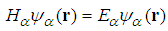
- Paper Submission
-
Journal Information
- About This Journal
- Editorial Board
- Current Issue
- Archive
- Author Guidelines
- Contact Us
International Journal of Theoretical and Mathematical Physics
p-ISSN: 2167-6844 e-ISSN: 2167-6852
2015; 5(5): 87-111
doi:10.5923/j.ijtmp.20150505.03
Some Solutions to the Fractional and Relativistic Schrödinger Equations
 Abstract
 Reference
 Full-Text PDF
 Full-text HTML
Yuchuan Wei
Department of Radiation Oncology, Wake Forest University, NC
Correspondence to: Yuchuan Wei, Department of Radiation Oncology, Wake Forest University, NC.
| Email: |  |
Copyright © 2015 Scientific & Academic Publishing. All Rights Reserved.
Laskin introduced the fractional quantum mechanics and several common problems were solved in a piecewise fashion. However, Jeng et alpointed out that it was meaningless to solve a nonlocal equation in a piecewise fashion and that all the solutions in publication were wrong except the solution for the delta function potential, which was obtained in the momentum space. Jeng’s critique results in a crisis of fractional quantum mechanics, that is, in mathematics it is quite difficult to find solutions to the fractional Schrödinger equation and in physics there is no realization for the fractional quantum mechanics. In order to eliminate this crisis, this paper reports some analytic solutions to the fractional Schrödinger equation without using piecewise method, and introduces the relativistic Schrödinger equation as a realization of the fractional quantum mechanics. These two sister equations should be studied at the same time.
Keywords: Fractional quantum mechanics, Fractional Schrödinger equation, Relativistic quantum mechanics, Relativistic Schrödinger equation
Cite this paper: Yuchuan Wei, Some Solutions to the Fractional and Relativistic Schrödinger Equations, International Journal of Theoretical and Mathematical Physics, Vol. 5 No. 5, 2015, pp. 87-111. doi: 10.5923/j.ijtmp.20150505.03.
Article Outline
1. Introduction
- In 2000, Laskin introduced the fractional quantum mechanics [1-3]. As the first example he solved the infinite square well problem in a piecewise fashion [3]. Since then, the piecewise method has been widely used in this field. In 2010, however, Jeng, et al [4] criticized that it was meaningless to solve a nonlocal equation in a piecewise fashion and they demonstrated thatit was impossible for the ground state function to satisfy the fractional Schrödinger equation near the boundary inside the well. In a series of papers [5-8], Bayin insisted that he explicitly completed the calculation in Jeng’s paper and the wave functions did satisfy the fractional Schrödinger equation inside the well. Hawkins and Schwarz [9] claimed that Bayin’s calculation contained serious mistakes. Luchko [10] provided some evidence that the solution did not satisfy the equation outside the well. On the other hand, Dong [11] re-obtained the Laskin’s solution by solving the fractional Schrödinger equation with the path integral method. It is not easyfor readers to judge their mathematical argument [12, 13], but weagree with Jeng that the piecewise method to solve the equation is wrong, since recently we explicitly and inarguably showed that the Laskin’s functions did not satisfy the fractional Schrödinger equation with
 anywhere on the x-axis [14]. According to Jeng, et al [4], only the solution for the delta function potential [15-17] was acceptable and they themselves provided a solution for the one dimensional harmonic oscillator potential for the case
  [4]. Readers have been looking forward to some other solutions to the fractional Schrödinger equation since the simple solutions for the infinite square well potential were disproved. Jeng et al [4] also showed their concern that there was no realization of the fractional quantum mechanics. Jeng’s critique resulted in a crisis within fractional quantum mechanics. In mathematics it is not easy to find a solution to the fractional Schrödinger equation, and in physics it is not easy to find realizations for the fractional quantum mechanics. In order to eliminate this crisis, this paper reports some solutions to the fractional Schrödinger equation without using the piecewise method, and introduces the relativistic Schrödinger equation [18-21], as a realization of the fractional quantum mechanics. Several solutions for the relativistic quantum mechanics are also presented.
 2. The Relativistic Schrödinger Equation: A Realization of the Fractional Schrödinger Equation
- In this section we will list the standard, fractional, and relativistic Schrödinger equations in one- and three-dimensional spaces, and explain why we claim the relativistic Schrödinger equation is an approximate realization for the fractional Schrödinger equation.
2.1. The Schrödinger Equation
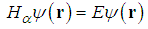
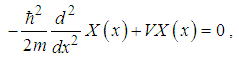
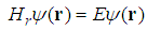
- In the standard quantum mechanics [22, 23], the time-independent Schrödinger equation is
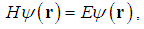 | (1) |
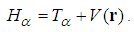
 is a wave function defined in the 3 dimensional Euclideanspace R3, E is an energy, and r is a vector in the 3 dimensional space. The Hamiltonian operator
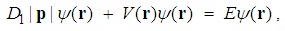
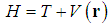 | (2) |
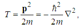 | (3) |
 is the momentum operator. As usual, m is the mass of a particle and
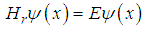
  is the reduced Plank constant.The one dimensional time-independent Schrödinger equation is
 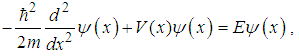 | (4) |
 and the potential
  are defined on the x-axis.
2.2. The Fractional Schrödinger Equation and Its Scaling Property
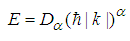
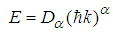
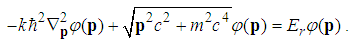
- In 2000 [1-3], Laskin generalized the classical kinetic energy and momentum relation (3) to
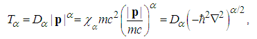 | (5) |
 is the fractional parameter, the coefficient
 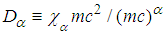 ,
,  is a positive number dependent on
  , and c is the speed of the light. Originally Laskin [1-3] ever required the fractional parameter
  , but in this paper we allow
  , as in [4, 9], with an emphasis on the simplest nonlocal case
  . In the case
  , taking
  , the fractional kinetic energy is the same as the classical kinetic energy
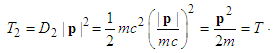 | (6) |
 , taking
  , the fractional kinetic energy is the approximate kinetic energy in the extremely relativistic case,
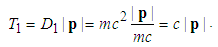 | (7) |
 | (8) |
 | (9) |
 | (10) |
 | (11) |
 , the fractional Schrödinger equation recovers the standard Schrödinger equation; when
  , the fractional Schrödinger equation is
 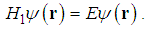 | (12) |
 , the following scaling property is straightforward. Scaling property. If a wave function
  and an energy E is a solution of the fractional Schrödinger equation for the potential
 | (13) |
 and
and  is a solution of the fractional Schrödinger equation for the potential
  , i.e.
 | (14) |
 is an arbitrary positive number. The proof is trivial. From (13) we have
 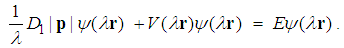 | (15) |
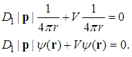
 , such as (1) the coulomb
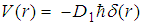
 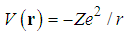 with the charge of an electron and Z the order number of an atom, or (2) the radial delta function potential
 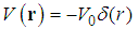 with the constant
  , the scaling property can be described simply as follows.Scaling property. For a potential
  with a property
 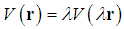 , if a wave function
  and an energy E is a solution of the fractional Schrödinger equation
 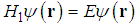 , then the wave function
  and the energy
  is also a solution. The one dimensional fractional Schrödinger equation is
 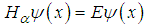 | (16) |
 | (17) |
 , we have
 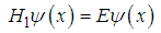 | (18) |
 | (19) |
 | (20) |
 denotes the convolution, and
  and
and  are generalized functions [25]. We point out that the generalized function
  is the well-known ideal ramp filter, which plays an important role in the theory and applications of Computed Tomography [26, 27]. We will discuss the relationship between fractional quantum mechanics and the computed tomography in another paper. The Dirac delta potential
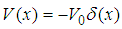
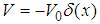
 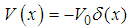 with
with  satisfies
 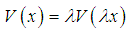 . Based on the scaling property, if a wave function
  and an energy E is a solution of the fractional Schrödinger equation
  with a delta potential well, then the wave function
  and the energy
  is also a solution. See Problems 3, 7, & 9.
 2.3. The Relativistic Schrödinger Equation
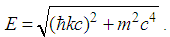
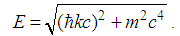
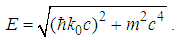
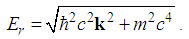
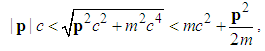
- According to the special relativity, the revised kinetic energy is [18]
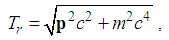 | (21) |

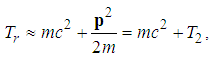 | (22) |

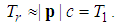 | (23) |
 will approximately correspond to a fractional kinetic energy
  , whose parameter
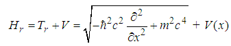
  changes from 2 to 1. Therefore the relativistic kinetic energy is an approximate realization of the fractional kinetic energy. The definition of the relativistic kinetic energy operator is
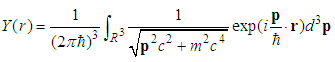
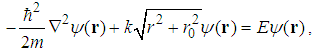
 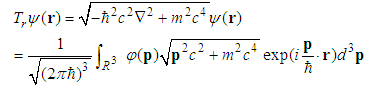 | (24) |
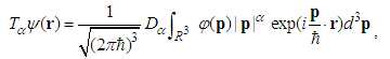
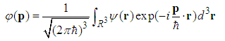
 is the wave function in the 3D momentum space. The relativistic Schrödinger equation is
 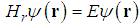 | (25) |
 | (26) |
 | (27) |
 | (28) |
3. Solutions to the Fractional Schrödinger Equation
- We will study the one dimensional problems first and then the 3D problems.
3.1. One Dimensional Problems
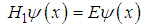
- Problem 1. (Thefree particle.)For
 , the fractional Schrödinger equation
  has the solutions
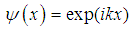 | (29) |
 | (30) |
 , or equivalently
 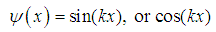 | (31) |
 | (32) |
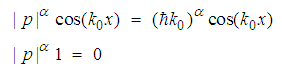
 . Proof. According to the definition of the fractional kinetic energyoperator [1-3], we obviously have
 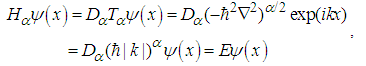 | (33) |
 . Further, for
  we have
 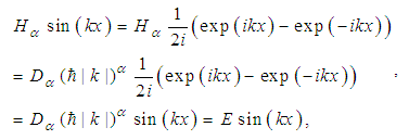 | (34) |
 | (35) |
 with V0 a constant, the eigen-functions do not change but the new eigen-energies become
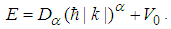 | (36) |
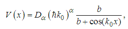 | (37) |
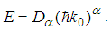
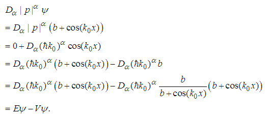
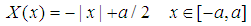
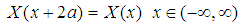
 , a is a positive real number (as throughout this paper), b is a real number, and
  , the fractional Schrödinger equation
  has a solution
 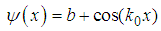 | (38) |
 | (39) |
 | (40) |
 | (41) |
 | (42) |
 | (43) |
 | (44) |
 | (45) |
 | (46) |
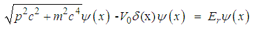
 with
with  , the fractional Schrödinger equation
  has a solution
 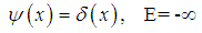 | (47) |
 | (48) |
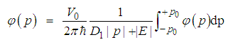
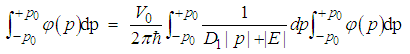
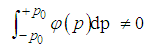
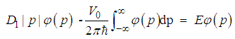 | (49) |
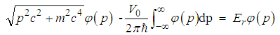
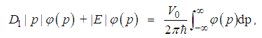 | (50) |
 is the wavefunction in the momentum space.We first change the integral limit in the above equation to a finite positive number
  , and then let
  . Thus we have
 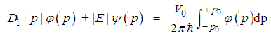 | (51) |
 | (52) |
 | (53) |
 | (54) |
 | (55) |
 | (56) |
 | (57) |
 | (58) |
 means that the wave functions at both sides are equal except for a constant coefficient. Obviously, a constant coefficient is not important for an eigen-wavefunction. Therefore we have
  | (59) |
 | (60) |
 | (61) |
 | (62) |
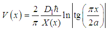
 ), as we will see soon.Problem 4. (The linear potential.)For a linear potential
  with
with  , the solutions to the fractional Schrödinger equation
  are
are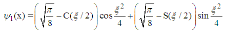 | (63) |
 | (64) |
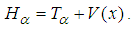
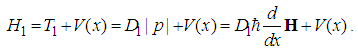
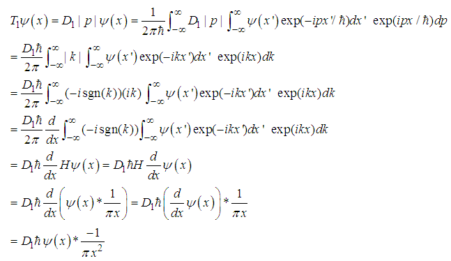
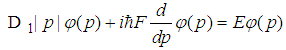
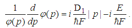
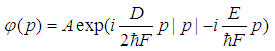
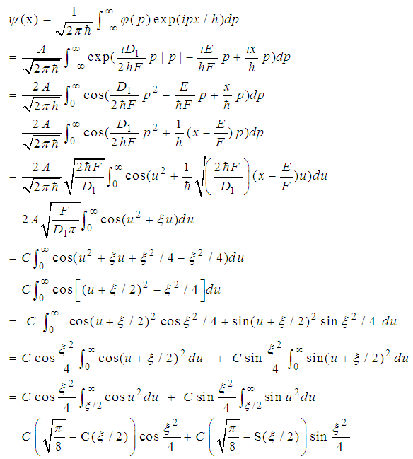
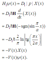
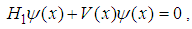
 .Proof.The fractional Hamilton is
 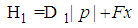 | (65) |
 | (66) |
 | (67) |
 | (68) |
 | (69) |
 | (70) |
 | (71) |
 | (72) |
 | (73) |
 | (74) |
 | (75) |
 | (76) |
 has the solution
 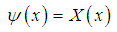 | (77) |
 | (78) |
 | (79) |
 | (80) |
 | (81) |
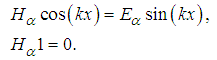
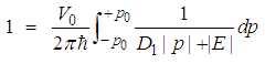
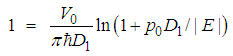
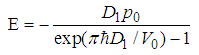
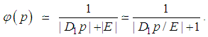
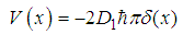
 with the Dirac comb potential
 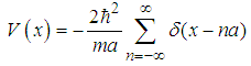 | (82) |
 | (83) |
 | (84) |
 | (85) |
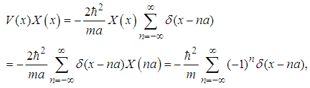 | (86) |
 | (87) |
 | (88) |
 has two and only two bound states
 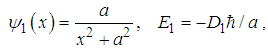 | (89) |
 | (90) |
 | (91) |
 | (92) |
 | (93) |
 | (94) |
 , we have
  | (95) |
 | (96) |
 | (97) |
 | (98) |
 | (99) |
 is the ground state, and
  is the first excited state. Since the excited energy
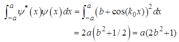
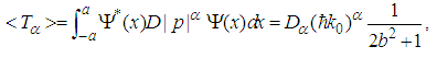
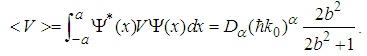
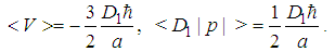
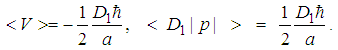
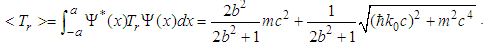
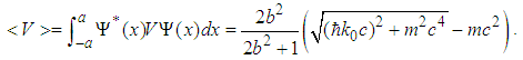
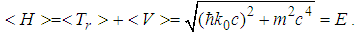
  , we know that there are no more excited states. The particle has only two bound states, the ground state and the excited state. This completes the proof.Let us further calculate the averages of the kinetic and potential energies in this elegant problem.The normalized functions are
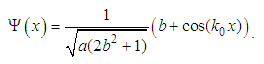
 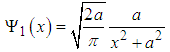 | (100) |
 | (101) |
 is even and
  is odd, the two states obviously are orthogonal, i.e.
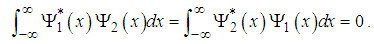 | (102) |
 | (103) |
 | (104) |
 | (105) |
 | (106) |
 | (107) |
 | (108) |
 , and notice that
 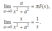 | (109) |
 | (110) |
 | (111) |
 | (112) |
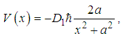
 has a bound state
  | (113) |
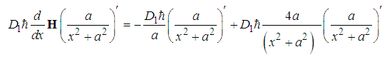 | (114) |
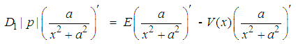 | (115) |
 | (116) |
 | (117) |
 | (118) |
 in Problem8, this statement follows immediately.
 3.2. Three Dimensional Problems
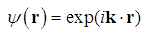
- Problem 10. (The Free particle.)For
 , the solutions for the fractional Schrödinger equation
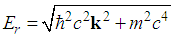
  are
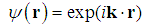
are | (119) |
 | (120) |
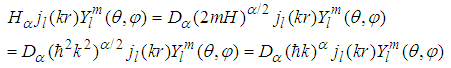
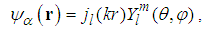
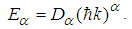
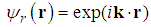
 any three dimensional vector. An alternative form of the eigen-functions is
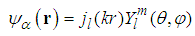 | (121) |
 is the spherical Bessel function of order l,
  is the spherical harmonic function of degree l and order m [22],
  is the spherical coordinate system, and
  is the length of the vector k.Proof. For
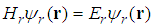
  , the standard Schrödinger equation
 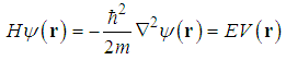 | (122) |
 | (123) |
 | (124) |
 | (125) |
 | (126) |
 | (127) |
 | (128) |
 | (129) |
 | (130) |
 | (131) |
 | (132) |
 | (133) |
 | (134) |
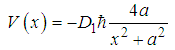
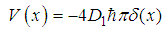
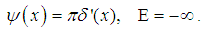
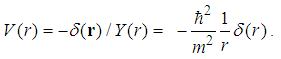
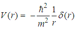
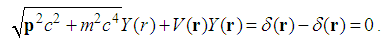
 with the potential
 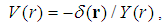 | (135) |
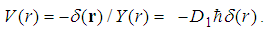
 is the Dirac’s delata function in the 3D space. Proof. It is easy to verify that
 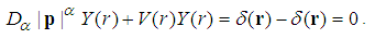 | (136) |
 we have
 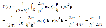 | (137) |
 | (138) |
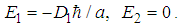
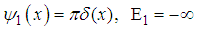
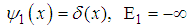
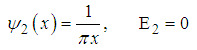
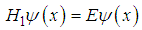
 , the Schrödinger equation
  has a solution
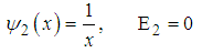
 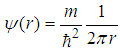 and E=0.(2) When
  , we have
 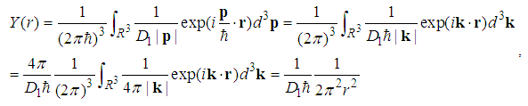 | (139) |
 | (140) |
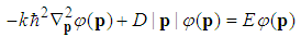
 , the fractional Schrödinger equation
  has a solution
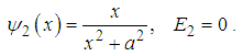
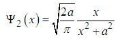
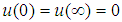
  and E=0. Problem 12. (The harmonic oscillator potential.)For a harmonic oscillator potential
 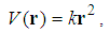 | (141) |
 has solutions(in the momentum representation)
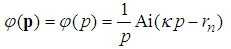 | (142) |
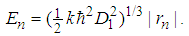 | (143) |
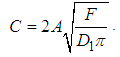
 is its n-th zero point, and
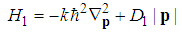
 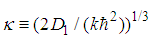 . Proof.The fractional Hamiltonian is
 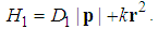 | (144) |
 | (145) |
 | (146) |
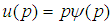
 is expressed as
  | (147) |
 , the eigen-equation becomes
 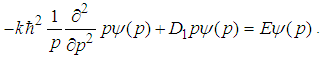 | (148) |
 . Then we have
 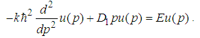 | (149) |
 is
is  | (150) |
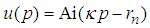 | (151) |
 is the Airy function,
  is its n-th zero point, and
 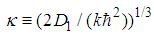 [4]. This completes the proof. Problem 13. (The Coulomb potential.)For the Coulomb potential
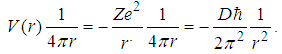
 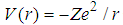 with Z>0, and e is the charge of the electron, the fractional Schrödinger equation has a solution
  with E=0 when
 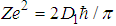 . Proof.In fact we have
 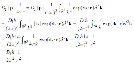 | (152) |
 | (153) |
 | (154) |
4. Solutions to the Relativistic Schrödinger Equation
- Again, let us study the one dimensional problems first and then the 3D problems.
4.1. One Dimensional Problems
- Problem i. (The free particle.)For V(x)=0, the solution for the relativistic Schrödinger equation
 is
is | (155) |
 | (156) |
 . Proof. According to the definition of the square root operator [18-20]
 | (157) |
 | (158) |
 | (159) |
 . Further, when V(x)=V0 with V0 a constant, the wavefunctions do not change but the new energy levels become
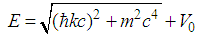 | (160) |
 | (161) |
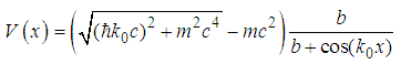
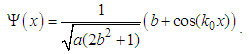
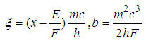
 , a is a length, and b is a real number, the relativistic Schrödinger equation
  has a solution
 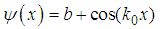 | (162) |
 | (163) |
 | (164) |
 | (165) |
 | (166) |
 | (167) |
 | (168) |
 | (169) |
 | (170) |
 | (171) |
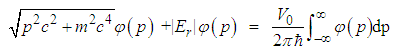
 with
with  , the relativistic Schrödinger equation
  has a solution
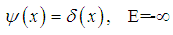 | (172) |
 | (173) |
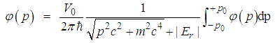
 | (174) |
 | (175) |
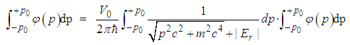
 , and then let
  . Thus we have
 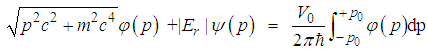 | (176) |
 | (177) |
 | (178) |
 , we have
 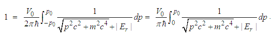 | (179) |
 , we have
 | (180) |
 | (181) |
 | (182) |
 | (183) |
 | (184) |
 | (185) |
 | (186) |
 | (187) |
 | (188) |
 | (189) |
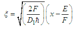
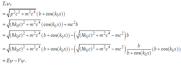
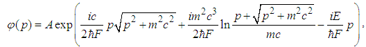
 with
with  , the solution to the relativistic Schrödinger equation
  is
is 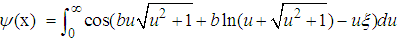 | (190) |
 | (191) |
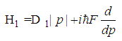
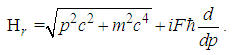
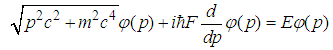
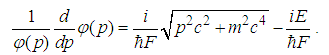
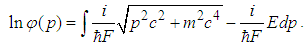
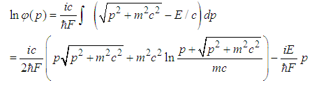
 .Proof.The relativistic Hamilton is
 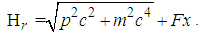 | (192) |
 | (193) |
 | (194) |
 | (195) |
 | (196) |
 | (197) |
 | (198) |
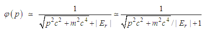
 is an arbitrary constant. Via Fourier transform, we can get the wavefunction in the real space
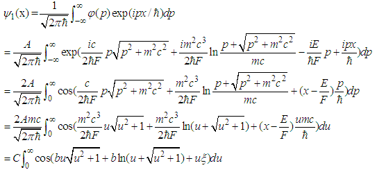 | (199) |
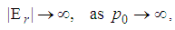
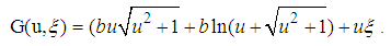
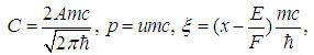 | (200) |
 | (201) |
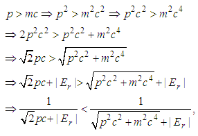
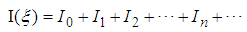
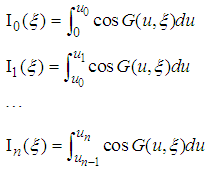
 is equal to the sum of an alternating series and the absolute values of the terms in the series become smaller when
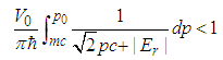
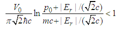
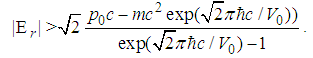
  . Specifically, let us consider the integral
 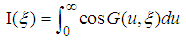 | (202) |
 | (203) |
 , suppose that
  with n=0,1,2,3 satisfy that
 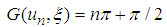 | (204) |
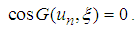 | (205) |
 | (206) |
 | (207) |
 alternately change their sign, and
 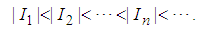 | (208) |
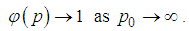
 converges for any given
  .As
.As  , the interval between any two adjacent points,
  , becomes closer to each other, every term
  , and hence their alternating summation
  . In other words, for any fixed
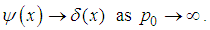
  , we have
 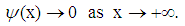 | (209) |
 , so we omit it temporarily. Interested readers can observe its behavior intuitively on a graph.
 4.2. Three Dimensional Problems
- Problem v. (The free particle.)For
 , the solutions to the relativistic Schrödinger equation
 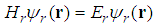 are
are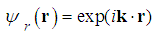 | (210) |
 | (211) |
 a three dimensional vector. An alternative form of the eigen-functions is
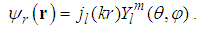 | (212) |
 , the standard Schrödinger equation
 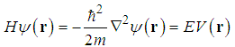 | (213) |
 | (214) |
 | (215) |
 is the length of the vector k.From the relationship between the relativistic Hamiltonian and the standard Hamiltonian
  | (216) |
 | (217) |
 | (218) |
 | (219) |
 | (220) |
 with the potential
 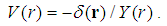 | (221) |
 | (222) |
 , the s-state energies for the relativistic Schrödinger equation,
  , satisfy
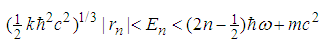 | (223) |
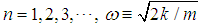 , and
, and  is the n-th zero point of the Airy function Ai(x).Proof.In the momentum space, we have
 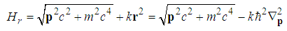 | (224) |
 | (225) |
 | (226) |
 | (227) |
 , but greater than the energy levels of the fractional energy with
  and
and  . Specifically, for s-state, we have
 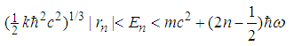 | (228) |
 Here we used the result of Problem 12 and the energy formula for the classical harmonic oscillator [22]. Problem viii. (The Coulomb potential.)For the Coulomb potential
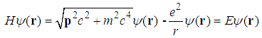
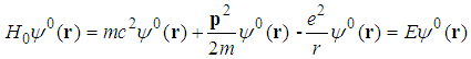
  , wheree is the charge of the electron, the energy eigen value of the relativistic Schrödinger equation
 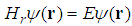 is
is 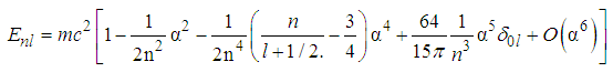 | (229) |
 is the fine structure coefficient, n is the principle quantum number, l is the angular momentum quantum number. Only in this problem and its solution,
  is not fractional parameter. Proof.The relativistic Hamiltonian is
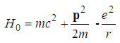
 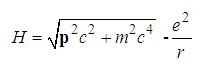 | (230) |
 | (231) |
 | (232) |
 | (233) |
 and energy levels
 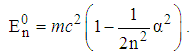 | (234) |
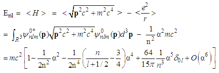 | (235) |
 | (236) |
 term, which is 41% of the observed Lamb shift [19]. We are trying to find the exact solutions for the relativistic Schrödinger equation with a Coulomb potential to see whether we can explain the Lamb shift better in the framework of quantum mechanics.
 5. Conclusions
- Jeng’s critique resulted in a crisis of fractional quantum mechanics, that is, the fractional Schrödinger equation was difficult to solve in mathematics and had no realization in the real world. To eliminate this crisis, we present various solutions to the fractional Schrödinger equation, and introduce the relativistic Schrödinger equation as a realization of the fractional Schrödinger equation. Several solutions to the relativistic Schrödinger equation are also presented. The standard, fractional and relativistic Schrödinger equation should be studied together. We wish that the winter of the fractional quantum mechanics could go away and its spring could come soon.
ACKNOWLEDGEMENTS
- The research on the relativistic Schrödinger equation was supported by Gansu Industry University (currently called Lanzhou University of Technology) during 1989-1991, with a project title ‘On the solvability of the square root equation in the relativistic quantum mechanics’.Cooperative research, joint grant applications and seminars on the new quantum mechanics are welcome.