Branko Mišković
Independent, Novi Sad, Serbia
Correspondence to: Branko Mišković, Independent, Novi Sad, Serbia.
| Email: |  |
Copyright © 2015 Scientific & Academic Publishing. All Rights Reserved.
Abstract
Fundamental equations of EM theory point to physical relations of space, time and motion of elementary particles and full cosmos. The two EM fields, their tensor and elementary forces, point to the temporal axis, as the fourth physical dimension. It is preferential amongst three spatial axes by its strict direction in 4D space. Poynting’s theorem, as 5D continuity equation of EM energy, demands the fifth axis, directed through material structure. On the bases of these insights, the global cosmic relations are elaborated, including the evolution of the cosmic process. The consideration of some empirical facts establishes the local relations of space, time and motion, strictly determining all the kinematical quantities, thus overcoming the arbitrary relativistic speculations.
Keywords:
Space, Time, Matter, Motion, Cosmos
Cite this paper: Branko Mišković, Space, Time and Motion, International Journal of Theoretical and Mathematical Physics, Vol. 5 No. 1, 2015, pp. 16-22. doi: 10.5923/j.ijtmp.20150501.03.
1. Introduction
Physics considers the laws of matter motion in the frames of space and time. These three natural categories cannot be strictly defined, but their intuitive senses are understood. 3D space and time, as the reference frame, form in common 4D space of mutually perpendicular axes. Apart the six degrees of freedom – in 3D, the phenomenal sequence of temporal instants may be understood as the compelled motion along the fourth axis. Unlike the spatial trinity of axes, arbitrarily oriented in amorphous space, the fourth axis is preferential by its exclusive direction in 4D. The local flows of a tenable substance (N) are described by the 4D continuity equation, ∇•(NV) + ∂tN = 0, consisting of the spatial and temporal terms. Possible extension of this equation – by a substantial term, in the sense of the formation and/or dissolution of the substance, points to respective new axis.Without any interpretation, Kant’s antinomy of the finite or infinite cosmos is overcome by Riemannian model of its circular axes, as if globally closed. However, this formal synthesis is not fully carried out. Cosmos is still understood as a limited domain in 3D, with its boundary surface and some cosmic background been behind it. Though the time beginning is at least implicitly associated with the big bang singularity, nobody had related its continual lapse with the further cosmic expansion. Any synthesis of Kant’s temporal antinomy, by the cyclic closure into itself of respective axis, has especially not been still proposed. Without convincing interpretations of space and time, some additional axes are also introduced speculatively. In the absence of the visible manifestation of a fifth axis, it is locally closed into itself on the structural level of elementary particles.The additional confusion is introduced by SRT, as the attempt of the inverse relation of space and time with each motion. Instead of possible global relations, on the cosmic level, space and time are related – in return, by the motion of each particular body or its subjective observer. By this artificial feed-back, the independent natural categories, as the frame of each motion, are conditioned by the arbitrary motion of each object and/or subject. Not only that a solid support in the causal sequence of the natural phenomena is thus lost, but space and time, with the events in them, are thus multiplied, as if determined by the various frames. This may be accepted as a set of subjective illusions, the distinct impressions of the same reality. However, SRT exceeds the frames of each experience, and of elementary logic – as the final frame of the common experience.EM theory related with mechanics and gravitation [1,2] opened the door for the global relation of space, time and motion. Starting from physical laws and their comparisons, these relations are established in the medium structure, finer from the phenomenal matter [3]. On the other hand, the considerations of the pretexts for SRT foundation [4], with the final uprooting of their logic, enable the exit from the contemporary scientific dead end. Instead of the impossible implicit relation of physics and psychology – on the mere phenomenal level, physical laws may point to more general logic of spiritual worlds [5]. Of course, this is mentioned as an incidental digression, the boundary orientation of physics. At least by conditional relation, on the global cosmic level, physics may be fully completed and finally united into the consistent natural science or philosophy.
2. EM Indications
The equations of EM theory point to the real temporal axis, curve 3D space and stratification of material structures along a new axis. These indications enable the foundation of a consistent and convincing 5D cosmology.
2.1. Elementary Interactions
The two EM fields were initially introduced via the force actions upon respective two dipoles (p & m): | (1) |
 | (2) |
Each field affects respective dipole by the torque turning it into the field course. The inhomogeneous fields produce the forces, drawing the dipoles into the stronger fields. All these effects are reducible to the field actions onto the two separate poles. This was the basis for the initial symmetry of the two fields, their objects and interactions.However, the symmetry is broken in the next step. Unlike phenomenal electric poles, p = qr, magnetic ones cannot be extracted from respective dipole. Instead, magnetic moment is obtainable by rotation of electric dipole around one of its two poles, according to the relation: m = qr × v.Though their external fields, determining their behavior, are similar, the internal fields are quite distinct. The electric field origins from the positive, and terminates on negative poles, but the external magnetic field is continued by the internal field, forming the common toroidal vortex. Unlike the apparent electric poles, as the field terminals, magnetic poles are transparent by their own field.Renouncing the transparent magnetic, let us compare the interactions of the apparent electric poles, in the form of the static (3a) and kinetic (3b) central laws:  | (3) |
 | (4) |
The particular kinetic interaction (3b), convenient for the comparison, understands the equal speeds of two poles, or the same speed of one moving pole – being affected by its own fields. The two factors of proportionality are strictly determined by (4). Unlike the mutual distance – in (4a), r – in (4b) – denotes the particle radius, as the distance of the surface charge from its own center. Of the two anti-symmetric laws, the former expresses the repulsion of equipolar charges, and latter – attraction of parallel currents. Unlike one or two particular speeds (V,v) – through 3D space, c denotes the common motion of all the particles along temporal axis. With the other opposite speed, the static law is the special case of kinetic one. More general kinetic law, at different speeds, we compare with respective two dynamic components: | (5) |
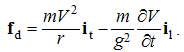 | (6) |
The former law concerns uniform motions, but latter of them acceleration, expressed in the general form of force action law, with g2 = 1 – (v/c)2, as the factor of the mass variation. Both transverse components are of magnetic, but longitudinal ones – of electric natures. The magnetic forces perform the kinetic interaction (5) or tend to the rectilinear motion (6). The electric forces complement the central form (5) or perform the energy transfer (6).
2.2. EM Fields
In the deductive approach, EM fields are defined from the two potentials, static (Φ) and kinetic (A):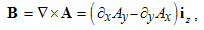 | (7) |
 | (8) |
Apart from the magnetic field, as the vortex of the kinetic potential in 3D, electric field is identified as the vortex of the generalized potential – in temporal planes, – under the formal condition: Φ= – At. Unlike the axial magnetic field, perpendicular to the vortex, the polar vector of electric field is defined in the vortex plane. In their essences, the two EM fields distinguish by their locations in 4D.The four Maxwell’s equations in the componential form can be expressed by the following pair: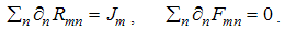 | (9) |
With the three current components in 3D, the fourth one represents the charge motion along t-axis. In the absence of free magnetic poles, (9b) lacks in free terms. The fields are identified by the following two tensors: | (10) |
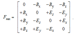 | (11) |
First rows and columns concern temporal, but remaining sub-tensor – spatial planes. The rational field locations, in the tensor (10), accords with (7) & (8), but that of the force fields, in (11), are opposite. They determine the two levels of observation, the former concerning the apparent electric, and latter – the transparent magnetic poles.Stratification of EM processes is expressed by Poynting’s theorem, as 5D continuity equation of EM energy, obtained from Maxwell’s equations: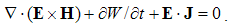 | (12) |
By spatial, temporal and substantial terms, this equation describes the energy motion through 5D space. The sources of the energetic current, in the first term, point to its flow through 3D space. The temporal derivative thus describes the energy density variation. The scalar product, E•J = F•V, represents the power density of the energy dissipation, as its transfer into the other structural layers.In this way, by means of EM theory, the fourth and fifth axes are here introduced, as the real physical dimensions. A few apparent antinomies, of the distribution of electric, and production of magnetic fields, further affirm the structural dimension, as the fifth, and Riemannian model of the curve, instead of the strait (Euclidian) exes.
2.3. Static Antinomy
Let us compare electric field around two charged surfaces, of a finite sphere and infinite plane, according to the static Maxwell’s equation: ∇•D = Q. In both cases, the fields are perpendicular to the charged surfaces. Radial electric field around the sphere declines by the square of the radius. On the spherical surface it equals to the surface charge. Due to the constant potential, the field inside the sphere equals to zero. However, with the same surface charge, the field of the plane, homogeneous in the surroundings, is divided into equal halves between the two sides. When its radius tends into infinity, the sphere turns into a plane. There arises the question of the field redistribution, from the sphere to the plane. This process is expected to be continual. Its interpretation is here illustrated by the implicit field distribution (Fig. 1), mutually reconciling and unifying the two distinct starting distributions.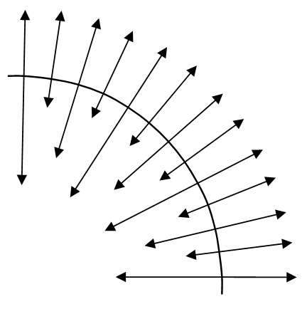 | Figure 1. Implicit field distribution |
This field is also equally divided between the two surface sides. Due to the same fields from all directions, the sum is annulled in the center. It has some value at all other internal points, up to the half of the charge surface. Not only that all components co-exist in the center, but continue towards the opposite surface, pierce it and add to the same external field, forming the full external value. By the way, it fully cancels the opposite internal field, thus reducing it to the zero of the phenomenal field distribution. The field redistribution just consists in its redirection. The implicit distribution on the figure does not take into account the final effect, from the opposite part of the spherical surface.Let us compare the two potentials. With constant internal static potential – of the zero field, its external value declines asymptotically, up to zero – at infinity. In the constant field of plane, the potential declines linearly, cut the abscissa and obtains negative values!? On the other hand, the constant potential would mean the zero field!The antinomy arises from the Euclidian geometry use. In the case of the curve space, the apparent plane is in fact the sphere, alike the circular Equator on the globe. Thus the field on both its sides takes the form of the internal field on Fig. 1. Starting from this hipper-equator, the potential tends to zero approaching each of the cosmic poles.
2.4. Kinetic Antinomy
According to the algebraic pair, H = V × D & E = B × U, one moving EM field produces the other, and vice versa. In accord with the differential set, convective variations of one, cause the other field in the resting medium. The validity of the algebraic equations is thus restricted to the motion in the field gradient direction. The motion of the central – electric, thus produces circular magnetic fields.This logic cannot be applied to a line current. Even if the moving field of the free electrons were separated from the opposite field – of the crystal lattice, there just remains the problem of the zero longitudinal field gradient. It can be overcome by returning to the set of elementary electric, and the sum of produced magnetic fields, existing in common at the same time and 3D location. According to the principle of Pauli, these fields occupy their own energetic levels, being arranged along the structural axis.
2.5. Material Essence
On the bases of the vortex (8) and tensor (10), the model of elementary charged particle is introduced, as the vortical displacement current, presented in [5].With respect to the dielectric medium and displacement current flowing through it, this vortex can persist only by its continual replacement along the t-axis. The internal and external flows, superimposed on the cosmic process, disturb the medium pressure, as the static potential. Its two signs accord with mentioned condition: Φ = – At .Similar vortex in 3D space represents a photon. In accord with EM theory, the two medium features (εμ) determine the same speed of propagation, c2 = 1/εμ, in both of the two directions in 4D. Restricted to the 3D space, as the moving medium, the light speed in 4D is c√2.There is neither the matter without motion, nor a motion without matter. Unlike the usual particle motion through 3D space, the perpetual propagation along temporal axis is the condition of material existence. In this way, the well-known philosophical idea is confirmed in the physical sense. It may be consistently related with cosmic expansion.
3. Global Motion
The discovery of red shift and its ascribing to the cosmic expansion opened the door for the relevant cosmology, with some quandaries concerning its elaboration. The most ideal extrapolation of this process in the past points to its possible singular start, in the form of a big bang. Its future prediction is a more difficult task. To avoid the expansion into infinity, some reasons for its redirection were looking for. However, this possibility is recently substituted by the unbelievable accelerated expansion into uncertainty.Instead of useless speculations, we here relate the lapse of time and cosmic expansion, with gravitation as a possible consequence. The compelled motion of matter along t-axis, determining the lapse of time, may be imagined in the form of the hipper-spherical wave. This idea gives the convincing interpretation of Riemannian cosmos. With circular spatial axes, its temporal thickness is reduced to a particle diameter and respective temporal instant:τ = 2rp/c.Starting from the center, cosmos attained the radius r = ct. The arc between two celestial bodies (d), as the 3D distance, depends on respective central angle (α): | (13) |
Its derivative gives the constant speed (v) of the mutual moving away. The ratio, d/v = t, inverse to the constant of Hubble, is the absolute time of the cosmic age. These relations understand the uniform cosmic process, as the wave propagating at the speed c, with provisional, less probable assumption of the straight temporal axis. In the case of this circular axis, the covered central angle (θ) must be taken into account: v = αc cos θIn this case, the decelerated cosmic expansion is expected to turn by time into the accelerated contraction. This prediction, however, contradicts to the increasing red shift.There remain the speculations with other forms of t-axis. The cosmic process in the Lobachevski’s form is similar to the toroidal particle model. Such a cosmos would overturn periodically, excluding the ideal cosmic singularities, as the big bang and big crash are. However, this is not the sole quandary. Instead of the assumed single wave, as a cosmic cunami, the periodical wave would represent a sequence of successive cosmoses. Even the two adjacent such cosmoses could not anyhow mutually communicate.There may be possible that the main physical constants vary in the expanding 3D medium. Unlike the cosmic wave, propagating through the restring solid 4D medium, the light propagates along this expanding wave. The expansion may cause the sparser medium, with respective variation of the speed of 3D light propagation. However, such effect would disturb the anti-symmetry of the laws (3).The introduced fifth axis is to be elaborated. Its definition can be founded on the structure zooming, expressed by the volume derivative (∂/∂v). Here the value ∂v represents the smallest relevant volume in the observed structural domain. It is conditioned by the structural elements, as the molecules, atoms and elementary particles – on one, and planets, stars and galaxies – on the other axis legs. As the smallest and greatest elements are not reached, the two axis legs are not restricted, but strive into opposite infinities.
4. Local Motion
4.1. Formal Relations
Under the pretext of the insolvable empirical difficulties, SRT does not admit the simultaneity or temporal relation of two distant events. However, such relations are usual in the astronomy. Following a distant object, its former position (r') is visible at the present time (t). With its known speed (v), present position (r) and former time (t') are calculated by help of the following two simple equations: | (14) |
Of course, the quantities are mediated by the finite speed of the light propagation. The interval (r'/c), between the light emission from the object and its detection on Earth, is determined by the distance r' and speed c.The similar transformation of the object position between two reference frames (15a) depends on the mutual motion. Here r' is the position in the frame moving at a speed v for the time t – in the comparative frame (r), starting from the common position of the two frames:  | (15) |
For the sake of formal symmetry, instead of the common time (t' = t), some its transformation (15b) was predicted. Not only that the lapse of time would depend on the mutual speed, but also on the comparative object position. However, unlike the former function conditionally predicted, the latter of the two variables is quite arbitrary.In fact, (15b) is introduced by the formal symmetry with the two field transformations: | (16) |
Moving through the field B – at a speed v, electric charge is affected by respective force, equivalent to the additional electric field: Ek = v × B. Expecting some symmetry of the analogous process, electric field would similarly affect the moving magnetic pole, equivalently to additional magnetic field: εμE × v. At least – in one direction, the analogous effect can be confirmed. Instead of the free poles, magnetic dipoles can be moved. With some technical restrictions, the relation (16b) is conditionally acceptable.The two cross-products point to the relevant fields being transverse to the object speed. The set (16) is of the inverse sense wit respect to (15): apart from the inverse functions of the two frames, electric field accords to the spatial, and magnetic – to temporal domains. These facts accord to the tensor (11), concerning magnetic carriers.The two sets (15) & (16) give the same set determinant, which would be entered into their inverse sets: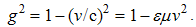 | (17) |
At the classical invariant time (t' = t) – instead of (15b), the determinant equals to unit. Moreover, the variable terms of (16) are annulled at the rest in the determined frame only, related with the medium. In other words, with respect to the square of speed in (17), the factor g is minimal just when the object rests in the preferred frame. All these facts point to the inequality of the two reference frames.The postulated equivalence of all (at least) inertial frames is formalized in SRT by re-division of the determinant, by g–1 – in the direct and inverse sets. This arbitrary correction deforms the transverse EM fields and thus calls in question Maxwell’s equations, as the field distributions. This fact is compensated by the complementary transformations of the two remaining, longitudinal and temporal axes: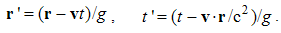 | (18) |
Although concealed by this new complication, the time dependence on the object position in the comparative frame further remains. Really, this formal inconsistency has not been noticed for a century of SRT existence.Mutual division of these transformations – (18a) by (18b) – gives respective speed transformation: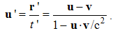 | (19) |
Here u = r/t is the speed in the comparative frame. In the case of light propagation, there follows the alluring formal result: c' = c. In fact, the postulated frame equivalence also includes the invariant speed of propagation.Although mathematically effective, this result cannot be anyhow inserted into physical reality. Its interpretation can be reduced only into the following equations: c – v = c, v = 0. With respect to the kinetic forces, dependent on speeds, the frame equivalence is restricted to the resting frames. With respect to the static forces, dependent on position, it must be finally restricted to only one preferred frame!
4.2. Empirical Facts
The invariance of light propagation is directly negated by the simple Doppler’s effects, at motion of the emitter (u) or detector (v). Testable at least for sound, the relations (20) can be generalized to each wave motion: | (20) |
Their two graphics are quite distinct. The former is the inclining hyperbola with the asymptote at u = c, and latter – declining straight line, with zero at v = c. The former fact points to possible wave wall in the emitter front, and latter – to the signal detection escape. Both functions depend on the variable wave speed on the device surfaces. In the cases of the celestial bodies, these processes are distributed in their fields. With respect to the cosmic distances, they may be also ascribed to the body surfaces.At the simultaneous motion (20) are mutually multiplied, thus giving (21a). If we associate the detector to emitter and substitute it by reflector, the radar equation (21b) would be actual. Here u is the radar speed, and v – of the reflector. The positive signs concern the reflected beam, propagating from the reflector towards radar: | (21) |
At relatively small speeds with respect to the propagation, the product uv may be neglected, and thus the function (21b) is reduced to only one variable: v' = v – u.As some geometric average, in the form of square root of (21b), the relativistic equation (22a) is formulated. As such, it is applied to all Doppler’s effects, including the red shift, more consistently described in [4] by (22b):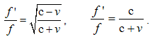 | (22) |
Both their diagrams decline by the speed of moving away of the two celestial bodies. Cutting the abscissa at v = c, the former function enables the possibility of the signal escape, which would be manifest by a horizon of the cosmic events. In the final instance, the moving away speed is restricted by the diameter of the expanding cosmos only. On the other hand, (22b) asymptotically approaches zero, excluding thus the mentioned (not noticed) cosmic effect. Both functions have vertical asymptotes, enabling thus the formation of the wave wall at possible cosmic contraction. However, evenly distributed red shift along the light path clearly points to its exponential function: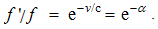 | (23) |
The avoidance of horizon demands the horizontal, and of the wall – the absence of vertical asymptotes. Amongst the three diagrams on Fig. 2, only (23) obeys both conditions, (22b) – only one, and (22a) – none of them. | Figure 2. Red shift diagrams |
With respect to the effects distributed in the gravitational fields, the speed of propagation is near to c on the surfaces of the massive celestial bodies. In the case of red shift only, it is invariant on the whole path, including the emitter and detector resting in the expanding 3D, but moving away – in 4D media. The relativistic generalization of these particular facts to each object/observer is finally denied by Sagnac’s effect, just dependent on the variable relative speed of light propagation. All the apparent indirect confirmations of SRT cannot be compared with this direct disprove.
4.3. Rational Interpretations
Michelson-Morley’s result is tried to explain at least by the three interpretations: 1) the ballistic hypothesis includes the emitter speed into light propagation, 2) Mach’s principle understands the objective orientation – with respect to the gravitational potential, as the local medium, and finally 3) Einstein’s postulate prefers the subjective orientations, with respect to the observers. First of them understands the mass of photons, the second – their wave nature, but third one is hesitating between the two interpretations.With respect to a photon, as the energetic particle, light does not manifest any inertia. Its toroidal model also obeys the wave speed of propagation. Even with the thesis of the twofold light nature, Einstein’s postulate denies (as if now rehabilitated) vacuum medium, understanding the multiple propagations of the same light, depending on the motion of various objects or their subjective observers.Some relation of gravitation and light propagation speaks in favor of Mach’s principle. From the law of gravitation, respective field and potential are defined: | (24) |
The field is directed towards the carrier. Its integration gives the potential, with the constant of integration (Xc), as the referent potential at infinity. Fig. 3 presents the potential against the radius starting from the center.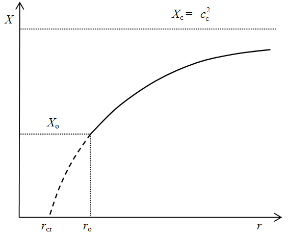 | Figure 3. Gravitational potential |
The potential is minimal at the body surface (ro), tending asymptotically to the maximal value (Xc) – at infinity. There is obvious that the potential dimensionally equals to speed square. Supposing the equality X = c2, the same diagram would present the speed of propagation.Possible body compression would reach the critical ratio, m/r = Xc/γ – of the zero potential, with full obstruction of the light propagation. This may be the case on a black hole surface and around it. At least qualitatively, the diagram accords to the known empirical facts. There is interesting its possible quantitative experimental testing.In the space between more celestial bodies, their fields add as the vectors, and potentials – as the scalars. A point between two celestial bodies, with the zero field, may have a respectable value of the potential. The referent potential (Xc) in practice accords to the location distant from these two, as well as from other celestial bodies. Forming the full medium of propagation, the fractional sum of all particular potentials determines the motion of the reference frame for light propagation:  | (25) |
Its motion with respect to the wider cosmic surroundings is determined by the speeds of relevant celestial bodies. The equivalent Fresnel’s factor (25b) determines the frame drag with a particular body. Michelson’s negative result is thus explained by predominant gravitational influence of Earth. Miller’s result may be ascribed to the influences of the other relevant bodies, as the Sun and full Galaxy.
5. Conclusions
The basic equations of EM theory locate the position and production of the two fields: magnetic – in 3D space, and electric – in temporal planes of 4D space. The comparisons of central forces, with confrontation of the empirical facts and theoretical results, determine an original, consistent and convincing cosmology, overcoming and negating SRT. The cosmos is reduced to a hipper-spherical balloon, expanding as the cosmic cunami along the temporal axis. The universal lapse of time is thus strictly determined. Riemannian curved model of 3D space is thus interpreted. Depending on the temporal axis form, the cosmic wave is projected into respective functions of the expansion. The linear expansion would give the cosmic age inverse to the Hubble’s constant. With respect to the increasing red shift, linear expansion may be substituted by Lobachevski’s open model of the temporal axis, in the toroidal form. This idea also excludes the cosmic singularities, as a big bang – in the beginning, or big crash – at the cosmic end.Going along the fifth axis, from the cruder to finer media, the greater speeds of the wave propagation, even above the speed of light (c), may be expected. With the finer waves and bigger speeds, the temporal direction of the propagation may be included. In a boundary case, with the infinite speed of the finest waves, each event would be simultaneously present in the whole cosmos, without medium disturbances. Full cosmos is thus reduced to a point, with the notions of space, time and motion finally overcome.
References
| [1] | B. Mišković, Axiomatic Presentation of EM Theory, SAP, Int. Journal of Electromagnetics and Applications, 2015. |
| [2] | B. Mišković, Fundamentals of Electrodynamics, SAP, Int. Journal of Electromagnetics and Applications, 2015. |
| [3] | B. Mišković, Medium of Natural Phenomena, SAP, Int. Journal of Theoretical and Mathematical Physics, 2014. |
| [4] | B. Mišković, Relativity and/or Symmetry, SAP, Int. Journal of Theoretical and Mathematical Physics, 2014. |
| [5] | B. Mišković, Final Essence of Material Existence, SAP, Int. Journal of Theoretical and Mathematical Physics, 2015. |
 Abstract
 Reference
 Full-Text PDF
 Full-text HTML