Raed M. Shaiia
Department of Physics, Damascus University, Damascus, Syria
Correspondence to: Raed M. Shaiia , Department of Physics, Damascus University, Damascus, Syria.
| Email: |  |
Copyright © 2014 Scientific & Academic Publishing. All Rights Reserved.
This work is licensed under the Creative Commons Attribution International License (CC BY).
http://creativecommons.org/licenses/by/4.0/

Abstract
In this paper, we will see that we can reformulate the purely classical probability theory, using similar language to the one used in quantum mechanics. This leads us to reformulate quantum mechanics itself using this different way of understanding probability theory, which in turn will yield a new interpretation of quantum mechanics. In this reformulation, we still prove the existence of none classical phenomena of quantum mechanics, such as quantum superposition, quantum entanglement, the uncertainty principle and the collapse of the wave packet. But, here, we provide a different interpretation of these phenomena of how it is used to be understood in quantum physics. The advantages of this formulation and interpretation are that it induces the same experimental results, solves the measurement problem, and reduces the number of axioms in quantum mechanics. Besides, it suggests that we can use new types of Q-bits which are more easily to manipulate.
Keywords:
Measurement problem, Interpretation of quantum mechanics, Quantum computing, Quantum mechanics, Probability theory
Cite this paper: Raed M. Shaiia , On the Measurement Problem, International Journal of Theoretical and Mathematical Physics, Vol. 4 No. 5, 2014, pp. 202-219. doi: 10.5923/j.ijtmp.20140405.04.
1. Introduction
Throughout this paper, Dirac's notation will be used.In quantum mechanics, for example [1] in the experiment of measuring the component of the spin of an electron on the Z-axis, and using as a basis the eigenvectors of  , the state vector of the electron before the measurement is:
 | (1) |
However, after the measurement, the state vector of the electron will be either  or
or  , and we say that the state vector of the electron has collapsed [1]. The main problem of a measurement theory is to establish at what point of time this collapse takes place [2].Some physicists interpret this to mean that the state vector is collapsed when the experimental result is registered by an apparatus. But the composite system that is constituted from such an apparatus and the electron has to be able to be described by a state vector. The question then arises when will that state vector be collapsed [1, 2]?Many interpretations of quantum mechanics have been offered to deal with this problem, and here, we will list a brief summary of some of them:The Copenhagen Intrepretation: When a measurement of the wave/particle is made, its wave function collapses. In the case of momentum for example, a wave packet is made of many waves each with its own momentum value. Measurement reduced the wave packet to a single wave and a single momentum [3, 4].The ensemble interpretation: This interpretation states that the wave function does not apply to an individual system – or for example, a single particle – but is an abstract mathematical, statistical quantity that only applies to an ensemble of similarly prepared systems or particles [5] [6].The many-worlds interpretation: It asserts the objective reality of the universal wavefunction and denies the actuality of wavefunction collapse. Many-worlds implies that all possible alternative histories and futures are real, each representing an actual "world" (or "universe") [7, 8].Consistent histories: This interpretation of quantum mechanics is based on a consistency criterion that then allows probabilities to be assigned to various alternative histories of a system such that the probabilities for each history obey the rules of classical probability while being consistent with the Schrödinger equation. In contrast to some interpretations of quantum mechanics, particularly the Copenhagen interpretation, the framework does not include "wavefunction collapse" as a relevant description of any physical process, and emphasizes that measurement theory is not a fundamental ingredient of quantum mechanics [9, 10].De Broglie–Bohm theory: In addition to a wavefunction on the space of all possible configurations, it also postulates an actual configuration that exists even when unobserved. The evolution over time of the configuration (that is, of the positions of all particles or the configuration of all fields) is defined by the wave function via a guiding equation. The evolution of the wave function over time is given by Schrödinger's equation [11, 12].Relational quantum mechanics: it treats the state of a quantum system as being observer-dependent, that is, the state is the relation between the observer and the system [13, 14].Transactional interpretation: describes quantum interactions in terms of a standing wave formed by both retarded ("forward-in-time") waves, in addition to advanced ("backward-in-time") waves [15, 16].Stochastic interpretation: it involves the assumption of spacetime stochasticity, the idea that the small-scale structure of spacetime is undergoing both metric and topological fluctuations (John Archibald Wheeler's "quantum foam"), and that the averaged result of these fluctuations recreates a more conventional-looking metric at larger scales that can be described using classical physics, along with an element of nonlocality that can be described using quantum mechanics [17, 18].Von Neumann–Wigner interpretation: It is an interpretation of quantum mechanics in which consciousness is postulated to be necessary for the completion of the process of quantum measurement [19, 20].The many minds interpretations: They are a class of “no collapse” interpretations of quantum mechanics, which is considered to be a universal theory. This means that they assert that all physical entities are governed by some version of quantum theory, and that the physical dynamics of any closed system (in particular, the entire universe) is governed entirely by some version, or generalization, of the Schrödinger equation [21]. In this paper, we will trod a different route in trying to solve the measurement problem.This subject of measurement in quantum mechanics was studied by many prominent scientists, including Heisenberg, von Neumann, Wigner and van Kampen [22]. And more recent studies such as the one done by Theo Nieuwenhuizen (Institute of Physics, UvA) and his colleagues Armen Allahverdyan (Yerevan Physics Institute) and Roger Balian (IPhT, Saclay), found that altogether, nothing else than standard quantum theory appears required for understanding ideal measurements. The statistical formulation of quantum mechanics, though abstract and minimalist, is sufficient to explain all relevant features. Since alternative interpretations involve unnecessary assumptions of one kind or another [22].In this paper, we will tread a different route in trying to solve the measurement problem. And we will start by contemplating, thoroughly, classical probability theory at first.When we toss a coin for one time, the sample space of this simple experiment is [23]:
 | (2) |
Of course, as it is known, this does not mean that the coin has all of these possibilities at once, it is merely a statement about the possible outcomes of the experiment. And after doing the experiment, we will get just one of these two results and not both. That means that one of the elementary events only will happen: either  or
or  , but not both at once [23].What if the state vectors were nothing but another representation of events in the sense of the usual classical probability theory? What if the state vector before measurement is just the representation of a sample space, and the result we get after measurement is just an ordinary elementary event, in a similar manner to the coin example, and in this sense the measurement is an experiment in the sense of the word used in probability theory? If we could reformulate classical probability theory in such a way that allows the representation of ordinary events by vectors, then this will lead to an entirely different understanding of the underlying mathematics of quantum mechanics, and hence to quantum mechanics itself. And this is the aim of this paper.
2. An Alternative Way to Formulate Classical Probability Theory
In this section we focus on the reformulation of probability theory, then we use this formulation in next section to reformulate quantum mechanics. We reformulate classical probability theory in a similar language to that is used in quantum mechanics. Later on, we show that this formulation reduces the number of postulates used in quantum mechanics.First we will start by considering finite sample spaces.Here it will be presented an outline of the method to be used in this formulation:Having an experiment with a finite sample space  , There is always a finite dimensional Hilbert space
  with a dimension equal to the number of the elementary events of the experiment.Then, we can represent each event by a vector in
  using the following method:I the square of the norm of a vector representing an event is equal to the probability of the event.II Given an orthonormal basis of
  , we represent each elementary event by a vector parallel to one of these basis vectors, such that no different elementary events are represented by parallel vectors, and the square of the norm of the representing vector is equal to the probability of the elementary event.III Then every event is represented by the vector sum of the elementary events that constitute it.From (I) we see that the vector
  representing the impossible event must be the zero vector because:
 | (3) |
So: | (4) |
And the vector representing the sample space must be normalized, because: | (5) |
Furthermore, we know that the probability of an event is equal to the sum of the probabilities of the elementary events that constitute it [23], for example if: | (6) |
So: | (7) |
So, are (I), (II) and (III) consistent with this rule? Actually they are. To see that, let us suppose that sample space is: | (8) |
And let us take some event  to be:
 | (9) |
Let us take the orthonormal basis  to represent the elementary events such that:
 is represented by
 | (10) |
Since  is a orthonormal basis, then it satisfies:
 | (11) |
 | (12) |
Where  is the identity operator.According to (III),
  must be represented by:
 | (13) |
Where in the last equation we did not write  because that would mean that
  which may not be the case in general.And by adopting the notation:
 | (14) |
 | (15) |
We have: | (16) |
Obviously, we see that  is represented using this basis as:
 | (17) |
As a result of (II) and (III) we see that  is represented by:
 | (18) |
And we see that: | (19) |
As an example that helps clarifying the former ideas, let us take the experiment to be throwing a fair die and the result to be the number appearing on top of it after it stabilizes on a horizontal surface.The sample space of this experiment is: | (20) |
Let us take  to be a orthonormal basis in Hilbert space, so:
 | (21) |
 | (22) |
Let us choose to represent the elementary event  by the vector:
 | (23) |
That means  is represented by:
 | (24) |
and the event  for example is represented by the vector:
 | (25) |
but the event  is represented by the zero vector.
2.1. The Algebra of Events
2.1.1. The Intersection of Two Events
The intersection of two events is an event constituted of the common elements of the two events [23] [24]. So, it must be represented by the vector sum of the vectors representing the common elementary events of the two vectors.For example, in the die experiment mentioned above, if we took the two events:  then
then  So:
So: | (26) |
 | (27) |
And: | (28) |
Now, we will prove a little result. Supposing the sample space of some experiment is: | (29) |
We see that for any event , we have: and
and  because
  . Now let us take two arbitrary events
  and
and 
 And let us suppose they are represented by:
 | (30) |
 | (31) |
Then we have: | (32) |
We notice that if  then all of deltas are zeros so
  .So, we get this result:
 | (33) |
We see that for any two events  and
and  , we can write the event
  as:
as: | (34) |
But since  then as we see according to (33) that:
 | (35) |
So: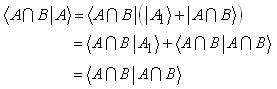 | (36) |
So: | (37) |
And: | (38) |
As a result: | (39) |
But since  , so:
, so: | (40) |
Or: | (41) |
So: | (42) |
And: | (43) |
Because  . And:
 | (44) |
We can write the former results, since the probability of some event is equal to the square of its norm, by the following manner: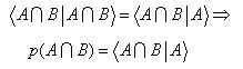 | (45) |
We see that: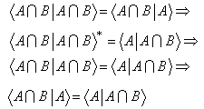 | (46) |
Finally, we can see also that, if we have two events: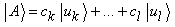 | (47) |
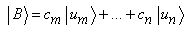 | (48) |
Then we can write the intersection of them as: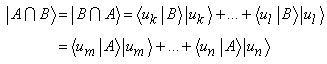 | (49) |
2.1.2. The Difference of Two Events
Let us take two events  and
and  . We saw from (34) that we can write the event
  as:
as: Where
Where  is an event constituted of elements not present in
  but belong to
  so:
so: That means:
 So:
So: | (50) |
We can see immediately that:
2.1.3. The Union of Two Events
We know that the union of two events is an event constituted of the elements belonging exclusively to the first one, the elements belonging exclusively to the second one and the common elements between the two [23] [24].So, it must be represented by: Which we can write as:
 | (51) |
Noting that: Because
  we can directly verify that:
 In a side note, we can prove that:
 So:
So: | (52) |
2.1.4. The Complementary Event
We know that the complementary event  of an event
  is given by [23] [24]:
 So:
So: So we have:
 | (53) |
We can directly verify that:
3. Observables
Let us suppose we have a system, and we want to do an experiment with it, which has the sample space: | (54) |
Or equivalently: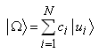 | (55) |
Where as we saw, since  is a orthonormal basis:
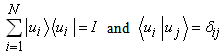 Now, if we take any
  real numbers:
 Then we can consider them to be the eignvalues of a Hermitian operator
  which is represented in this basis by the matrix:
 Clearly, the vectors of the ordered basis
  are the eignvectors of
  which satisfy:
 | (56) |
From the fact that this is true for any lambdas, in other words the values of  are arbitrary, then the vectors of the basis
  are the eignvectors of an infinite number of Hermitian operators in Hilbert space.Not even just that, but since this is true for any lambdas, then whenever we assign real numbers to elementary events, we can consider them to be the eignvalues of some Hermitian operator in Hilbert space corresponding to the eignvectors
  .And since the observable is by definition a function from the elementary events to real numbers [1], then we can represent any observable we define on the system, by a Hermitian operator in Hilbert space.But we have to be careful here: all the observables we have talked about have the same set of eignvectors, and we will call them compatible observables, and if we take any two of them, we find that their commutator is zero, because they have the same eignvectors.If we take one of these observables, let it be
  , which is represented by:
 Then we can think of the experiment as giving us one eignvalue of the observable. And since this is true for every one of the compatible observables with
  as we saw, then it is clear that compatible observables can be measured simultaneously together with a single experiment, which is the experiment we talked about.Now, let us suppose that:
 | (57) |
Which means that  is degenerate with a degeneracy
  .. That means we will get
  in the experiment if we get
  ,
, ,
, , or
, or  . In other words, if the event:
  happened.So:
 | (58) |
So we see, that if  was degenerate, then it is probability is equal to the probability of the projection of
  on the subspace spanned by the eigenvectors corresponding to
  . So, each eignvalue of the observable is represented by a subspace so to speak.But what about other observables we can define on the system corresponding to other experiments? Those experiments may have in general totally different probability distributions, which means the probabilities of their elementary events are different of those in the experiment we have talked about in the beginning of this section. Even more, the number of the elementary events may be different.Let us suppose we have a system. And let us assume that we intend to do some experiment on the system which has the sample space:
 | (59) |
Or equivalently: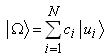 | (60) |
Now we will divide all the experiments we can do on the system into classes of experiments. Each class is composed of experiments that have the same number of outcomes (the same number of elementary events). So the experiment that we talked about is one member of the class  where
where  is the class of experiments that have
  elementary events by definition.We will name our experiment
  . We saw that for the experiment
  , we can define an infinite number of compatible observables (Hermitian operators) which all have the same eignvectors
  . Let us now take another experiment from the same class
  which we will call
  . What we mean by another experiment on the system is that we cannot do
  and
and  simultaneously.Let us suppose the sample space of
  is:
is: | (61) |
Now in general, the probability distribution of  may be radically different from that of
  . So, how are we going to represent the events of
  by vectors? Well, since we can represent
  by a vector in any N-dimensional Hilbert space, then we can represent it in the same Hilbert space that we used to represent
  . We can use another basis in this space and use another vector (different from
  ) to represent
  , or we can use the same basis and a different vector from
  to represent
  , or we can use a different basis (different from
  ) and the same vector
  to represent
  , where the components of
  on the new basis are which determine the probabilities of the events of
  . All these approaches are valid, but we will choose the last one (we could also have worked in a different Hilbert space all together). Of course we can represent
  with the same basis and the same vector for the sample space, if it has the same probability distribution of
  . But to distinguish
  as an experiment that cannot be done simultaneously with
  , we will represent its elementary events by a different basis.Now for
  , we have:
 | (62) |
As in the case of  , here, we can define an infinite number of observables (Hermitian operators), all compatible, and which have the eignvectors
  , and those observables are associated with
  . Since all of them have the same set of eignvectors, then the commutator of any two of them is zero.But if we take one of them, let it be
  , and take an observable
  associated with
  , then since
  and
and  do not have the same eignvectors (because
  is not
  ), then
  .And since
  and
and  cannot be done simultaneously, then we cannot measure
  and
and  simultaneously, because each observable is defined in terms of the experiment it is associated with. So we call them incompatible. Now, before we continue, let us take some examples of some compatible and incompatible observables.1-Compatible observables:In the experiment of throwing the die, we can define the first observable to be the number appearing on the top side of the die, and the second observable to be the square of the number appearing on the top side of the die.Let us call the first
  and the second
  . We have:
 | (63) |
Where: | (64) |
We have: | (65) |
And: | (66) |
So  is represented by:
 | (67) |
While  is represented by:
 | (68) |
We see that: | (69) |
2-Incompatible observables:Let us take a coin. We will imagine two ideal experiments that we can do with it. In the first, let us call it  , we toss the coin and it stabilizes on a horizontal surface and the top side of it is either Heads or Tails. We can define the observable
  to take the value 1 for Heads, and the value -1 for Tails. The second experiment,
  , is throwing the coin in a special way, that makes it stabilizes on its edge on some horizontal surface. We suppose that the edge of the coin is half painted. We can define an observable
  to take the value 1 if we looked at the coin from above and saw the edge either all painted or all not painted, and -1 if we saw it partially painted. We see that we cannot do both
  and
and  simultaneously, so:
  .*(Notice that for some class of experiments
  , once we used a vector to represent the sample space of some experiment, then we have to ask ourselves, can we use it to represent all the sample spaces of all the experiments of this class that can be done on the system?Clearly, when we want to represent the sample space of some experiment by a vector in Hilbert space, we can choose any Hilbert space that has the right dimensionality, and any orthonormal basis in it to represent the elementary events, and a vector to represent the sample space that satisfies that the squared norms of its components are the probabilities of elementary events. But after this if we want this vector to represent all the experiments of this class, we have to choose the bases representing those experiments carefully. Or we can choose the bases that represent all experiments in Hilbert space, then look for the vector that can be used as a sample space vector for all of them.And as we will see in the future, not every vector we use to represent the sample space of some experiment of some class, satisfies this for all experiments of the given class. So, we will call any vector that actually satisfies this condition, meaning it represents the sample space of all possible experiments of a given class that can be done on the system, we will call it the state vector of the system because it gives us the information about any experiment we can do on the system for a given class of experiments. And from now on, throughout this paper, when we use the term "state vector", we mean it in this particular sense. We will talk more about this later).Now, what if we take two experiments from different classes, say
  and
and  where
where  ? Let us suppose that the experiment
  is from the class
  and
and  is from the class
  . Here we will represent each experiment in its own Hilbert space:
  in
in  and
and  in
in  .Let us suppose we represent the sample space of
  in
in  by:
by: | (70) |
And that we represent the sample space of  in
in  by:
by: | (71) |
Now, let us suppose that we do both experiments on the system. Even more, we will suppose that doing either experiment does not affect the probability distribution of the other, whatever the order of doing the two experiments, was.When we do  , we have the sample space:
 | (72) |
Let us suppose that after doing  we do
we do  and that for
  the sample space is:
 | (73) |
Let us take the composite experiment  that is doing
  then
then  on the system. The sample space of this experiment is:
 | (74) |
Where we know that, if the probability of  in
in  is
is  and the probability of
  in
in  is
is  then the probability of
  is [24] :
 | (75) |
That is interesting, because if we take the vector space: | (76) |
and take the vector  in it which is:
 | (77) |
Where by definition: | (78) |
First of all, we see that the dimensionality of  is
is  . If we considered
  to be the vector representing the sample space of some experiment that has
  elementary events, then the probability of the elementary event
  is:
is: | (79) |
Well, it is the same probability of the event  in the experiment
  which has a
  elementary events. From the above we see that we can represent the sample space of the composite experiment
  by a vector
  in the Hilbert space
  where:
 | (80) |
Where the elementary event  is represented by
  .Now, what if doing one experiment affects the probability distribution of the other? Here, we can still write the sample space of the composite experiment as:
 | (81) |
Because the outcomes of the two experiments remain the same, but what is changing, is probability distributions. So, we cannot write:  because finding
  is not independent from finding
  in general.Still, the outcomes of the composite experiment are
  elementary events, so we have to represent
  in a Hilbert space with
  dimensionality. And any Hilbert space with this dimensionality will do. So, we can represent
  in:
in: And since we can choose any orthonormal basis in it, and since
  are orthonormal basis, so we can represent
  by:
by: | (82) |
Where  and
and  representing the elementary event
  , thus:
 | (83) |
We can generalize this to any number of experiments.P.S. when we define the sample space of some experiment, it is not necessary that we really do the experiment, but it just describes a potential experiment.Now, let us ask ourselves a question: is the state vector unique? Can we represent it for a given class, with another vector/vectors?If it is not unique, then we must find the same probabilities for all experiments of this class that we can do on the system, whether we used  or –if exist- the other state vector/vectors that can be used as state vectors.Let us suppose that for an experiment
  , the state vector of the system is written as:
 | (84) |
Let us replace the vector  by the vector
  which is:
 | (85) |
Where  are complex numbers which we will write in the form:
 | (86) |
Where:  . for
. for  to be a state vector for the system, then all the probabilities of the elementary events (so all the probabilities of all events since the probability of an event is the sum of the probabilities of its elementary events) of any experiment from this class must be the same as given by
  . So, the probabilities of the elementary events of
  do not change.So the following equation must hold:
 | (87) |
So: | (88) |
And because the former condition is true even if we choose the experiment to satisfy:  for all values of
  , because our choice of
  is arbitrary, we must have:
 So we have the condition:
 | (89) |
Which means that: | (90) |
And that: | (91) |
But that is not enough, because the condition that probabilities must not change must be true for any other experiment from the same class we can do on the system and not just  , because we are talking about state vectors here.Let us take another experiment
  of the same class. We know that it must be represented by another basis, let us say
  . We must have:
 | (92) |
We have: | (93) |
Where: | (94) |
For  we must have:
 | (95) |
So: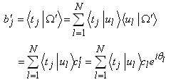 | (96) |
We saw that the probabilities of the events of  do not change. But to reach our goal, which is that we want
  to be a state vector too, then the probabilities of the events of
  must not change. So, we must have:

 So we must have:
 | (97) |
The former equation must be true for any  and
and  because we are speaking of arbitrary experiments with arbitrary probability distributions. It is true when we fix the basis whatever
  were. So their coefficients must be the same (we fixed the two bases and can define an infinite number of experiments on them):
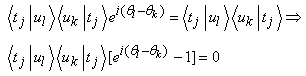 | (98) |
It must be true for all experiments so for all bases even when:  for any
  and
and  . So:
. So: So:
So: 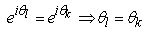 | (99) |
And that is for any  and
and  . So we have:
 | (100) |
So we see that: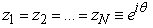 | (101) |
So: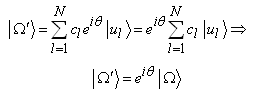 | (102) |
So, for  to be a state vector too, it must be of the former form. From the above we see that we can multiply
  by any pure phase without changing anything.
4. The Collapse of the State Vector
Let us suppose that we have a system. We want to do on it an experiment  of the class
  . That means the state vector of it is:
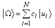 | (103) |
Let us suppose that the result of the experiment was  , which means that the elementary event
  has happened. Let us suppose that we want to do another experiment now on the system from the same class, after we did the first one.Well, one such experiment could be just reading the result of the former experiment. Since the result was
  then definitely we will find the result
  . So we can represent the sample space of this experiment by:
 | (104) |
But, according to the note  , the state vector after the measurement i.e. after doing the second experiment (after reading the result), must be able to represent this experiment. So it must give the same probabilities for the elementary events of this experiment. So we must have:
 | (105) |
Which means the state vector after the measurement must be of the form: | (106) |
we can use this vector to represent any other sample space of any experiment of the same class  , which we do after the measurement, because it is the state vector after the measurement.So, if the state vector before we do some experiment was given by (103), and after that, we did the experiment and got the result
  , then the state vector of class
  after the measurement becomes:
 | (107) |
Of course we can choose any value for  including
  so we can write the state vector after the measurement as:
 | (108) |
We can call this a collapse in the state vector. But we also see that there is nothing mysterious here, for we just have a change in probability distribution after the measurement.We can see that another way to express the above is, that if  is an observable that the experiment measures (as we have mentioned that means a Hermitian operator that has
  as its eigenvectors), then the system after the measurement will be in an eigen state of
  corresponding to the eigenvalue of it that we will measure.
5. Entangled States
Now, how do we represent composite systems?Let us at first take two non-interacting systems. Let us do an experiment  on the first one of the class
  (
( is the class of experiments we can do on the first system with
  outcomes). Its sample space will be of the form:
 | (109) |
and we will suppose the state vector of it is: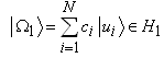 | (110) |
And let us suppose that the sample space of the second experiment  on the second system of the class
  is:
is: | (111) |
and we will suppose its state vector is | (112) |
We know that the sample space of the composite experiment  of doing
  and
and  together is:
 | (113) |
We see that  has
has  outcomes.Even more, since the two systems do not interact with each other, the then probability of the result
  is:
is: | (114) |
Where  is the probability of getting
  in the experiment
  , while
  is the probability of getting
  in the experiment
  .We know that we can represent
  in any Hilbert space of dimensionality
  by a vector that gives the elementary events of
  the former probabilities.If we take the vector:
 | (115) |
We see that  has the dimensionality
  . Furthermore:
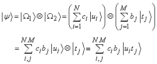 | (116) |
We see that: | (117) |
So, we can use  as a representation of the sample space of some experiment with
  outcomes. Furthermore, the basis vector
  can represent an elementary event with a probability:
 | (118) |
From all that we see that we can use: | (119) |
to represent  with
with  representing the elementary event
  .And since we are working in a new space altogether, we can use this vector to be the state vector of the composite system, taking into account that we have to be careful after it, to choose the bases representing other experiments of the class
  on the composite system in the right way.We can call
  a product state.We can take as an example of the above two non-interacting fair coins. The sample space of the experiment of tossing a first coin is:
 | (120) |
and let us suppose that its state vector before measurement was: | (121) |
And for the second coin: | (122) |
And we suppose too that its state vector: | (123) |
And the sample space of the composite system (tossing the two coins together) is: | (124) |
So the state vector for the composite system of the two coins is: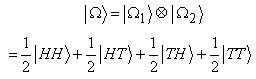 | (125) |
P.S: we see that writing sample space as a vector is more expressive, because it does not show only the results, but it shows their probabilities too.Now: what if the two systems were interacting with each other?Here, we can still write the sample space as given by the equation (113), and that is if the outcomes of the two experiments remain the same, but what interaction is changing, is probability distributions. So, we cannot write: 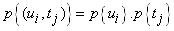 because finding
  is not independent from finding
  in general.Still, the outcomes of the composite experiment are
  elementary events, so we have to represent
  in a Hilbert space with
  dimensionality. And any Hilbert space with this dimensionality will do. So, we can represent
  in:
in: | (126) |
And since we can choose any orthonormal basis in it, and since  are orthonormal basis, and we are working in a whole new space
  different from both
  and
and  , thus we can represent the state vector of the composite system by:
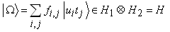 | (127) |
Where  and
and  representing the elementary event
  .We see that the product state is a special case of the former formula when
  .We call any state
  an entangled state if it is not a product state.Now we can talk about the composite (system-observer) system.
6. The Observer-system Composite System
Let us start by an example, then generalize. Let us take the composite system of (coin-coin tosser). The sample space of the coin is: | (128) |
And we will suppose its state vector is: | (129) |
The observer (coin tosser) may get two results: observer seeing the coin Heads, or observer seeing the coin Tails. So, the sample space of the experiment which is the observer observing the coin is: | (130) |
And let us suppose its state vector is: | (131) |
Bearing in mind that: | (132) |
And that: | (133) |
So, we have: | (134) |
The state vector of the composite system (which can be thought of as the sample space of the experiment of observing the composite system of coin – coin tosser) as we know, can be written as: | (135) |
But we know that we can only get either  or
or  , so:
, so: | (136) |
Even more, the probability of the observer sees it Heads is the same as the probability of getting Heads. The same goes for tails. So: | (137) |
So: | (138) |
So,  is an entangled state. In the same way, if we have a system with a state vector:
 | (139) |
Then each  corresponds to an elementary event of the observer which has the same probability, so it can be represented by
  where:
 | (140) |
and the state vector of the observer is: | (141) |
And the state vector of the composite system (which is the sample space of the experiment that is observing the composite system) is of the form: | (142) |
But since the probability of the event  is zero when
  so:
so: | (143) |
And we have: | (144) |
We can write  as:
as: | (145) |
Where: | (146) |
So, the measurement is an entanglement between the system and the observer.
7. Time Evolution of Systems
The physical state of the system might change with time, so that means the state vector describing it might change with time, because the probability distributions of experiments might change with time. We will talk about time evolution of closed systems at first. First of all, what is the definition of a closed system? We will adopt the following definition:A closed system is a system which satisfies that its characteristics are independent of time, meaning, when we study the system, it does not matter where we choose the origin of time, as long as we do not do a measurement on it.Since the number of outcomes is the same in any moment of time we want to do the experiment, so at time  we can represent the state vector of the experiment in the same vector space that we represented the state vector of it at time
  .We know that each observable is represented by a Hermitian operator, and the experiment we do to measure it has its events represented by orthonormal basis that is the eigenvectors of this operator. We will keep the bases representing all the experiments the same, and see how must the state vector change with time to keep satisfying that it is the state vector for the closed system. So, for the observable
  that
that  are its eigenvectors we can keep them the same, but then the state vector might change in general. So the state vector at time
  is of the form:
 | (147) |
Where  is the time elapsed after the moment
  .We will search for a linear operator
  such that, if we start the system in any initial state
  , then its state after a time
  is given by:
 | (148) |
But since the state vector is a sample space vector, hence it is normalized, so: | (149) |
So: | (150) |
We see that we can accomplish that by choosing  to be unitary:
 | (151) |
Where  is the identity operator. So we will choose
  to be a unitary operator.Furthermore, from (148) we see that:
 | (152) |
It is a well known fact [1] that from the equations (151) and (152) in addition to (148) we can deduce that: | (153) |
Where: | (154) |
which means that  is a Hermitian operator. Now, what about unclosed systems? We have to find an equation that describes the system in general, whether closed or not, and which becomes identical to (153) when the system is closed. For this, we can define an operator
  for each system that satisfies:
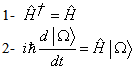 3- When the system is closed,
  is deduced from a unitary evolution with time of the state vector.
8. Treating a Simple System as a Composite System
If we have a system, and  is an experiment of the class
  that we can do on it, and the state vector for the experiments of this class for this system is:
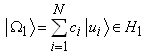 | (155) |
While  is another experiment we can do on the system, and it is of the class
  where
where  . Where we assume that the state vector of this system for this class of experiments is:
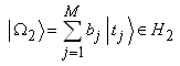 | (156) |
Each experiment has its probability distribution, which we will assume it is independent from the other experiment. As we saw, the sample space vector of the composite experiment  which we can do on the system which is doing
  then doing
  on it is:
 | (157) |
And since it is a vector in a  dimensional Hilbert space, then we can consider it as the state vector of the system for the class
  ensuring of course that we represent the experiments of this class by the bases that ensures that
  is a state vector.But from the above we see that we can think of the system as equivalent to two separate non-interacting systems where the state vector of the first is given by (155), and the state vector of the second is given by (156). So the state vector of the composite system will be given by (157), since they are non-interacting:
9. Continuous Probability Distributions
What if we want the experiment to tell us about the position of some particle? Clearly, the way we used when talking about representing events by vectors is of no use here, because we are dealing with continuous probability distributions. So, we have to update our tools a little.We will work first with a special example, then generalize. Let our example be a particle moving on a line.Here, we will represent events by vectors in an infinite dimensional Hilbert space, because we have infinite values of  . And in this space, we will represent the observable
  by the operator
  , which satisfies:
 | (158) |
And we will demand the inner product in this space to satisfy: | (159) |
Furthermore, we demand this inner product to satisfy also:For any  and any well behaved complex function
  :
: | (160) |
 | (161) |
Where:  .We can write any
  as:
as: | (162) |
Because then: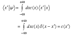 | (163) |
So: | (164) |
We can define  where:
  , as:For any
  :
: | (165) |
 | (166) |
So:  :
: | (167) |
So we have: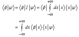 | (168) |
With all of that being said, now we can represent events as the following:We represent the event: | (169) |
(where  and the intervals
  might be open, closed or half open/half closed and we have a finite number of them, let us call it
  ) by a vector
  in some infinite dimensional Hilbert space
  as follows:1.
  2.
2.  We know that:
 Thus:
Thus: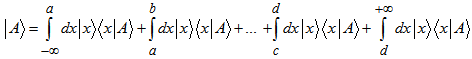 | (170) |
But all integrals except the ones in which are over intervals spanned by the event  are equal to zero because in the intervals that do not satisfy that we have
  so:
so: | (171) |
Where we are integrating only over intervals spanned by  and this is the meaning we will give to the former equation throughout this paper. We can see that:
 | (172) |
Since: | (173) |
That yields: | (174) |
Now: | (175) |
But from (174) we know that: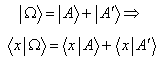 | (176) |
We know that when  we have:
  so substituting in (176) gives:
 | (177) |
Using the former equation in (175) we get: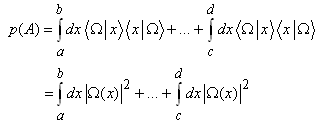 | (178) |
Where: | (179) |
So the probability of being in the interval  is:
is: so
so  is the probability density.We can generalize this process to any continuous observable. And if we want to measure another incompatible observable, we do as we did in the case of discrete variables, meaning we represent it by another basis. It is fairly easy to generalize for three dimensions.Also here, we will represent events by vectors in an infinite dimensional Hilbert space. And we will suppose that there is in this space the vectors
  which satisfy:
 | (180) |
Where: | (181) |
Where the integration over the whole of space and  is the position vector of the particle, and
  is the infinitesimal volume around
  . Furthermore we demand the inner product in this space to satisfy:For any
  and any well behaved complex function
  :
: | (182) |
 | (183) |
Where  may be all of space or only some part of it.And we define
  where
where  may be the whole of space or only some part of it, as follows: for any
  :
: | (184) |
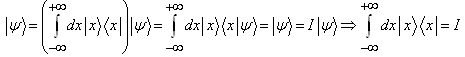
 | (185) |
From all of the above we can prove, in a similar manner to what we did in the one dimensional case, that:For any  and
and  we have:
 | (186) |
 | (187) |
 | (188) |
Where the integration extends over all of space, and  is the identity operator.With these tools, we can continue exactly as we did in the one dimensional case.
10. Quantum Mechanics
Now with these concepts at hand, we need no assumptions in quantum mechanics, just we need to apply them. We will take as an example the component of the spin of an electron along the z-axis [1].If we created an electron somehow, in general, when we turn on a magnetic field in the z-direction, we might find the component of the spin of the electron either up or down with a certain probability depending on the initial state. If the electron was originally up or originally down, then we find it after turning on the magnetic field certainly up/down as is known [1]. But there are states that we sometimes get up and other times get down so they are different than the electron being up or being down before we turn on the magnetic field [1]. So how do we explain that according to the new formulation of classical probability theory? In this new interpretation of quantum mechanics, we see that quantum mechanics is just a statistical theory in the same way classical experiments are. To understand the experiment of measuring the component of the spin of an electron, we will compare it to a classical experiment which is measuring the Headness or the Tailsness of a coin. What we mean by the statement: the result of the experiment is Heads/Tails, is that after we toss the coin, the upper surface of the coin after it stabilizes on a horizontal surface is Heads/Tails. So, before tossing the coin, i.e. when it is still in my hand, there is no meaning of the question "is the coin Heads or Tails?". All we can talk about is the sample space of the experiment. And in this case we saw that the state vector of the coin (which represents the sample space) is of the form: | (189) |
Now, after tossing the coin, we have some definite result, either Heads or Tails. And as we saw before, we can represent the sample space vector of any experiment of the same class that we can do on the coin after tossing, i.e. the state vector after the measurement, by (if the result was say Heads): | (190) |
Which means that if we read the result of tossing, we will find it definitely Heads.In the same way, before turning the magnetic field on, there is no meaning of the question "is the component of the spin of the electron up or down?" but the state vector before the measurement (which represents the sample space) of measuring the component is of the form: | (191) |
But after turning on the magnetic field, we will have a definite result, let us say up, so the state vector after the measurement can be written as: | (192) |
And that represents the sample space for any experiment of the same class after the measurement.
11. What about Bell's Theorem?
In fact this new interpretation is in total agreement with Bell's theorem.As we saw when we spoke of incompatible observables, they are in this interpretation, observables that cannot be measured in the same experiment. And that any two observables that their commutator is not zero are incompatible.Furthermore, we saw that if the sample space of the experiment is not already an eigenvector of the observable we want to measure, then there is no meaning of the question "what was this property before doing the experiment?". So, when we have two electrons in the singlet state, and since according to this interpretation, the state vector in the singlet state is nothing more than a representation of the sample space of the experiment of measuring the spins of the electrons, and this sample space is represented by: | (193) |
It means that we cannot say before measuring the spins that the spins were opposite because it is like saying the coin is Heads while it is still in my hand.Also, the three components of the spin of an electron are represented by incompatible observables, so they cannot be measured together. And since there is no meaning of what is the component before measuring it, so we cannot say that the three components of the spin of the electron can have values together.From all of the above we see that Bell's theorem is actually in favour of this interpretation and supports it.
12. Implications
Of course, we see that if this interpretation is true, then it can replace some of the currently existing interpretations of quantum mechanics. Furthermore, this interpretation needs no special requirements in quantum physics and sees it as an inevitable result if we consider all properties of particles to be statistical, i.e. if nature is indeterministic, and hence the overwhelming number of quantum mechanical axioms become results of this new formulation of classical probability theory and not axioms derived from experiments.Since space is represented by operators (position operators) in quantum mechanics, so before measuring them, they have no meaning, according to this interpretation. Still, the system that we are studying exists. So, according to this interpretation, and in order for it to be true, space must be an emergent property. So, there must be deeper ways to describe matter. And the laws of quantum mechanics are the statistical laws governing this un spatial state. So, maybe this state has its own laws that may be non statistical and that are even deeper than quantum mechanical laws. Moreover, if we take two entangled particles, let us say two electrons in the singlet state, so the state vector is given by the equation (193). This means that before the measurement they are neither (the first up and the second down), nor (the first down and the second up), as the coin when it is still in my hand is neither Heads nor Tails.If we separated these two electrons by a great distance, then do the measurement, so measuring one will surely affect the other because their spins will become opposite. How this happened? Well, this link between them that is deeper than space which we have talked about, suggests that it may provide the answer by allowing particles to exist and interact in a level deeper than space itself.Also, with this new understanding of quantum concepts, we see that quantum systems are not as different as we thought before from the classical systems. The only difference is that we assume that all properties of quantum systems are statistical, but we do not tend to think about classical systems that way. Anyway, we can apply the concepts of superposition, entanglement and the collapse of state vectors on some aspects of classical systems as we saw, which imply that we can use some classical systems as Q-bits that are much more easily to manipulate, and hence may make quantum computation more practical.There is another problem that we can bypass using this interpretation. If we take two electrons in the singlet state which is given by (193). Then when we measure them, we find that they simultaneously assume opposite spin components along the Z-axis (for short we will say they assume opposite spins). But we know from special relativity that simultaneity is relative. So, according to which observer this word “simultaneously” is referring [25]? In fact, we have no contradiction between special relativity and quantum mechanics here at all. The reason is, that here, we should not talk of two events –the first spin assumed the value up and the other assumed the value down (not necessarily in this order)- rather, here we have one event which is doing the experiment in the sense of the word used in probability theory (because as we saw the outcomes of an experiment are not recognised until we do it). And doing the experiment in this interpretation is doing the measurement. And when we do an experiment in probability theory and get some particular result, then we can say that the result is one event that comes from doing the experiment. And we can in a looser language say that this event (getting the result) is the same as doing the experiment. In the same sense, we say that after doing the measurement on the two electrons in the singlet state, then what we get is one event and not two events. But we know from special relativity that different observers agree on events, but in general disagree on how to mark them with spatial and temporal coordinates. So this event –the collapse of the state vector of the composite system (which means that after measurement the electrons assume opposite spins)- is an event that all observers agree that it happens in this way. What they could disagree on is where or when it happened.Another result of this interpretation is that it proves that if we have any indeterministic universe, which can be described using probability theory, and in which the properties of its elementary particles are indeterministic in this manner, then the laws that govern this kind of universe must be those of quantum mechanics. And hence the answer to the question: “why are the laws of our universe the way they are?” may be: “because our universe is indeterministic”.
ACKNOWLEDGEMENTS
I wish to acknowledge Diaa Fadel and Ammar Atrash for their help in typing this document.
References
| [1] | http://theoreticalminimum.com/courses/quantum-entanglement/2006/fall. |
| [2] | Quantum Mechanics - an Introduction, 4th ed. - W. Greiner. |
| [3] | http://abyss.uoregon.edu/~js/21st_century_science/lectures/lec15.html. |
| [4] | https://www.princeton.edu/~achaney/tmve/wiki100k/docs/Copenhagen_interpretation.html. |
| [5] | Quantum Mechanics: A Modern Development - Leslie E. Ballentine. |
| [6] | The Ithaca interpretation – N. D. Mermin. |
| [7] | Hugh Everett Theory of the Universal Wavefunction, Thesis, Princeton University, (1956, 1973), pp 1–140. |
| [8] | Everett, Hugh (1957). "Relative State Formulation of Quantum Mechanics". Reviews of Modern Physics. |
| [9] | R. B. Griffiths, Consistent Quantum Theory, Cambridge University Press, 2003. |
| [10] | Omnès, Roland (1999). Understanding Quantum Mechanics. Princeton University Press. |
| [11] | Bohm, David (1952). "A Suggested Interpretation of the Quantum Theory in Terms of 'Hidden Variables' I". Physical Review. |
| [12] | David Bohm (1957). Causality and Chance in Modern Physics. Routledge & Kegan Paul and D. Van Nostrand. |
| [13] | Finkelstein, D.R.: "Quantum Relativity: A Synthesis of the Ideas of Einstein and Heisenberg"; Springer-Verlag; 1996. |
| [14] | Laudisa, F.: "The EPR Argument in a Relational Interpretation of Quantum Mechanics"; Foundations of Physics Letters. |
| [15] | The Transactional Interpretation of Quantum Mechanics by John Cramer. Reviews of Modern Physics. |
| [16] | An Overview of the Transactional Interpretation by John Cramer. International Journal of Theoretical Physics. |
| [17] | Edward Nelson (1966). "Derivation of the Schrödinger Equation from Newtonian Mechanics". Physical Review. |
| [18] | Khavtain Namsrai (1985). Nonlocal Quantum Field Theory and Stochastic Quantum Mechanics. Springer. |
| [19] | Wigner, Eugene; Henry Margenau (1967-12). "Remarks on the Mind Body Question, in Symmetries and Reflections, Scientific Essays". American Journal of Physics. |
| [20] | Chalmers, David (1996). The Conscious Mind: In Search of a Fundamental Theory. Philosophy of Mind Series. Oxford University Press, USA. |
| [21] | http://www.bss.phy.cam.ac.uk/~mjd1014/ommi.html. |
| [22] | http://phys.org/news/2013-07-physicists-publish-solution-quantum-problem.html. |
| [23] | An Introduction to Probability Theory and Its Applications, volume I – William Feller. |
| [24] | Fundamentals of Probability and Statistics for Engineers – T. T. Soong. |
| [25] | The Fabric of The Cosmos, chapter 4 - Brian Greene. |

 Abstract
 Reference
 Full-Text PDF
 Full-text HTML