B. Ita1, P. Tchoua2, E. Siryabe3, G. E. Ntamack3
1Department of Pure and Applied Chemistry, University of Calabar, Cross River State, Nigeria
2Department of Mathematics and Computer Sciences, University of Ngaoundere, Ngaoundere, Cameroon
3Department of physics, Group of Mechanics and Materials (GMM), University of Ngaoundere, Ngaoundere, Cameroon
Correspondence to: P. Tchoua, Department of Mathematics and Computer Sciences, University of Ngaoundere, Ngaoundere, Cameroon.
| Email: |  |
Copyright © 2014 Scientific & Academic Publishing. All Rights Reserved.
Abstract
A generalized series is used to obtain bounded solutions of the Klein Gordon equation using the Frobenius method. For some examples used, we obtain similar results to that using Nikiforov Uvarov method (NU). Our approach is very simple and can solve many problems where the Nikiforov Uvarov method (NU) fails.
Keywords:
Klein Gordon Equation, Frobenius Method, Nikiforov Uvarov method, Bound State Solutions
Cite this paper: B. Ita, P. Tchoua, E. Siryabe, G. E. Ntamack, Solutions of the Klein-Gordon Equation with the Hulthen Potential Using the Frobenius Method, International Journal of Theoretical and Mathematical Physics, Vol. 4 No. 5, 2014, pp. 173-177. doi: 10.5923/j.ijtmp.20140405.02.
1. Introduction
Many of the physical phenomena of nature are characterized by some basic differential equations. For example, quantum mechanical phenomena are described by Schrodinger’s equation, which dictates the dynamics of some quantum systems represented by a Hamiltonian operator. One is primarily interested in finding all eigenvalues and eigenstates of such Hamiltonians. As a consequence, finding a large class of analytically exactly solvable quantum systems is an important goal and this search has already been initiated by Schrodinger using the factorization method [1, 2]. Recently, there has been renewed interest in solving simple quantum mechanical systems within the framework of the Nikiforov-Uvarov (NU) method [3]. This algebraic technique is based on solving the second-order linear differential equation which has been used successfully to solve Schrodinger, Dirac, Klein-Gordon and Duffin-Kemmer-Petiau wave equations in the presence of some well-known central and non-central potentials [4-13]. In this paper, our focus is to deal with the Klein Gordon equation with Hulthen potential.This paper is organized as follows: after a brief introduction in section 1, we give the review of the NU method and in section 2, we present the Frobenius method. In section 3 we solve the Klein Gordon equation by the NU method and in section 4 we use the Frobenius method to solve the same equation. Finally the two solutions obtained are compared and conclusions drawn.
2. Review of the Nikiforov-Uvarov Method (NU)
The Nikiforov-Uvarov (NU) method reduces the second order linear differential equation to a generalized equation of hypergeometric type. Using an appropriate coordinate transformation S = S(r), the equation takes the form: | (1) |
Where  and
and  are polynomials of at most second degree and
  is a first degree polynomial.By taking the following factorization
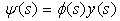 | (2) |
Equation (1) reduces to the hypergeometric type equation in the form: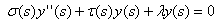 | (3) |
Where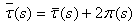 | (4) |
Ans satisfies the condition 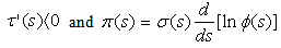 | (5) |
The parameter  , is defined by:
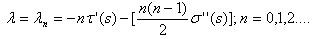 | (6) |
To determine the eigenvalues of energy, we need first to determine  by using the first derivative of
  and defining by:
 | (7) |
By solving the resulting quadratic equation for  , we obtain the following expression:
 | (8) |
The determination of is the essential point in the calculation of  and it can be obtained by setting the discriminant of the square root to zero.The Wave function in the relation (2) can be determined using the Rodrigue’s relation:
 | (9) |
Polynomial solutions  are given by:
 | (10) |
 is the normalization constant and the weight function
  satisfies the following relation:
 | (11) |
3. Review of the Frobenius Method
This method finds the solutions of a differential equation in the form of series, either a whole series, a Laurent series, or even a series involving contribute exhibitors. The difference between these situations is the properties of regularity of the equation coefficients. To do this you must put the equation in the form: | (12) |
Suppose a regular singular point  , singular functions
  and
and  and using the Fuck’s theorem, we can write the solutions of the differential equation in the form:
 | (13) |
The indicial equation is obtained for  | (14) |
For each found values  , we determine the values
  and then the solutions of the differential equation.
4. Application of the Nikiforov-Uvarov (NU)
Let us consider the following Klein Gordon equation in polar coordinates. The three dimensional radial wave equation of the KGE is written as | (15) |
Where the wave function is 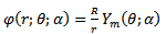 E is the relativistic energy, M the mass of the particle's spin-zero and
 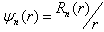 the wave function. The Hulthen potential is given by
  .Using the condition S (r) = V (r), the radial Klein-Gordon equation becomes:
 | (16) |
Taking into account the transformation  , the equation (16) becomes:
 | (17) |
with  ,
,  and
and | (18) |
Comparing equation (17) to equation (1), we get the following polynomials: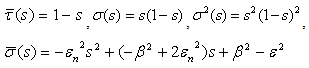 | (19) |
By replacing these polynomials by their values in the equation (8), one obtains: | (20) |
 | (21) |
To check the conditions of the polynomial 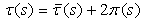 , we will take as values:
 | (22) |
 | (23) |
If we combine these with  defined in equation (7), we obtain the following expressions:
 | (24) |
And  | (25) |
Using equation (6), we have: | (26) |
Using the condition  , i.e. tying the equations (25) and (26), one obtains the eigenvalues of
  as:
as: | (27) |
Equations (18) and (27), one obtains the eigenvalues of energy given by: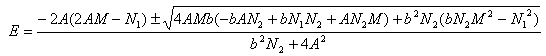 | (28) |
The polynomial solution of the hypergeometric function y (s), depends on the determination of the function  . Using the differential equation (11) we have:
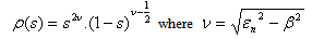 | (29) |
By substituting equation (29) in Rodrigue’s relations given in equation (10), one obtains: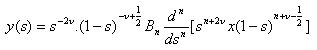 | (30) |
Equation (30) may come in the form of Jacobi polynomials [23] according to the following relationship: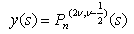 | (31) |
The Jacobi polynomial  is given by [23]:
 | (32) |
We can therefore write the equation (31) in the following form: | (33) |
where  is the Pochhammer symbol [23].For the determination of
  we solve equation (9), using the calculated values for
  and.
and.  . we obtain:
 | (34) |
Replacing  and
and  by their values in the equation (2), we obtain:
 | (35) |
With  and
and  is the normalizing constant.
5. Application of the Frobenius Method
Consider the same Klein-Gordon equation and the same Hulthen potential given in section 2. After development, we get the following equation: | (36) |
Using the condition  ,
,  , equation (36) becomes:
 | (37) |
Ask  and
and  , equation (37) becomes:
 | (38) |
By using the Fuck’s theorem, we can write: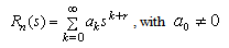 | (39) |
Differentiation gives us: | (40) |
Equation (40) in (38), one obtains: | (41) |
By effecting a change of variable, we obtain: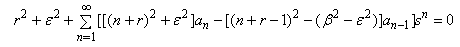 | (42) |
By solving the indicial equation  , we obtain:
 | (43) |
For  , we have:
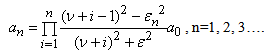 | (44) |
So it gets a representation of the solution. | (45) |
Using the relations (36) and (43), we obtain the energy E eigenvalue associated with the wave function. We can express the solutions obtained based on the Jacobi polynomial: this result is more accurate. The coefficients of the solution being assessed explicitly, we seek bounded solutions. We will only retain the negative value. In one of our papers in preparation, an explicit relationship between the solutions obtained by Nikiforov and Frobenius method is established. We also establish that the coefficients of the solution by the Frobenius method may be obtained by the differential transform method (DTM).
6. Conclusions
In this paper we have constructed exact solutions of the Klein Gordon equations by the NU and the Frobenius method. The energy eigenvalues are estimated and the coefficients of the Frobenius series estimated: The exact relation between the solutions obtained by the two methods is to be established in a fort coming paper
References
| [1] | A. Soylu, O. Bayrak and Bostosun, Chin. Phys. Lett. 25, 2754(2008). |
| [2] | S. H. Dong, Commun. Theor. Phys. 55, 969(2011). |
| [3] | S. M. Ikhdair, J. Quant. Infor. Sci. 1, 73(2011). |
| [4] | L.Z. Yi, Y.F. Diao, J.Y. Liu and C.S. Jia, Phys. Lett. A. 333, 212(2004). |
| [5] | X.C. Zhang, Q.W. Liu, C.S. Jia and L.Z. Wang, Phys. Lett. A. 340, 59(2005). |
| [6] | W.A. Yahya, K.J. Oyewumi, C.O. Akoshile and T.T. Ibrahim, J. Vect. Rel. 5. 27(2010). |
| [7] | H. Motavaiii and A. R. Akbarieh, Int. J. Theor. Phys. 49, 979(2010). |
| [8] | L.H. Zhang, X.P. Li and C.S. Jia, Phys. Lett. A. 372. 2201(2008). |
| [9] | N. Rosen and P.M. Morse, Phys. Rev. 42, 210(1932). |
| [10] | C.S. Jia, T. Chen and L.G. Cui, Phys. Lett. A. 373, 1621(2009). |
| [11] | T. Chen, Y.F. Diao and C.S. Jia, Phys. Scr. 79, 065014(2009). |
| [12] | J. Sadeghi and B. Pourhassan, EJTP. 5, 193(2008). |
| [13] | Y.F. Cheng and T.G. Dia, Phys. Scr. 75, 274(2007). |
| [14] | A.N. Ikot and L.E. Akpabio, accepted in Applied Physics Research (APR). |
| [15] | O. Yesiltas and R. Sever, arxiv: quant-ph/0703034. |
| [16] | B.M. Mandal, Int. J. Mod. Phys. A15, 1225(2000). |
| [17] | N. Saad, Phys. Scr. 76, 623(2007). |
| [18] | A. Arda and R. Sever, Int. J. Theor. Phys. 48, 945(2009). |
| [19] | W. Greiner, (Relativistic Quantum Mechanics, Berlin, Springer, 1990). |
| [20] | A.F. Nikiforov and V.B. Uvarov, (Special Functions of Mathematical Physics, Birkhaiiser, Basel, 1988). |
| [21] | E.D. Filho and R.M. Ricotta, Phys. Lett. A340, 388(2005). |
| [22] | C. Tezcan and R. Sever, Int. J. Theor. Phys. 48, 337(2008). |
| [23] | S.I. Gradshteyn and I.M. Ryzhik, Table of Integrals, Series and Products, Seven edition (Elsevier Academic Press, USA, 2007). |
| [24] | A.N Ikot, Oladunjoye and B I Ita (Few Body System 2012) Springer Verlag. |
| [25] | Harun et al(Physica Scripta59;1999). |
| [26] | B.Falaye et al; Chin Phys.B Vol 22 No.11(2013). |
| [27] | Abdalla et al; Rep Math.Phys.71(2013). |
 Abstract
 Reference
 Full-Text PDF
 Full-text HTML