1. Introduction

Understanding the physics of the phase diagram of the superconducting cuprates has remained one of the outstanding problems in condensed matter physics since the discovery of high T_C in these materials. The expectation has always been on the possibility of understanding the origin of the superconducting phase in order to possibly design room temperature superconductors. The superconducting phase of the cuprates is a manifestation of new mechanism of interaction of the material carriers when they are properly doped. One of the consensus from all these years of intense study of the superconducting cuprates is that their electronic phase diagram is the same [1-6]. As the temperature is reduced from about 300 K which is near room temperature (297 K), the superconducting cuprates show signs of the superconducting state, even though their conductivity is ordinary. The general believe is that a superconducting state evolves when the electrons pair up to form Cooper pairs and are propagated coherently. The difference in the energy of the Cooper electrons and the so-called free electrons is called the energy gap. Thus one classic sign of superconductivity is the emergence of an energy gap which is a range of energy levels that are forbidden to electrons, with all states below the gap completely filled [7-9]. In conventional low-temperature superconductivity, the presence of this gap signifies the sudden transition to the superconducting state at T_C. However in the case of the high-temperature superconductors, a similar energy gap also occurs under certain circumstances above the transition temperature when the parent materials are slightly doped. This onset of a gap at higher temperature designated T* (T-star) that is far above T_C, is generally called a pseudogap. Thus the pseudogap is a set of anomalous physical properties below the characteristic temperature T* and above T_C [10-13]. Condensed matter physicists hope that understanding this shadow of the superconducting state will shed light on the mechanism for high T_C superconducting cuprates [1, 13-17]. There are basically two schools of thoughts here. The first school believe that as the temperature is lowered, first reaching T*, a few electron pairs start to form, but they are sparse and lack the long-range coherence for the Cooper pair condensate propagation. It follows that as the temperature continues to fall, more such pairs are formed until, upon reaching T_C, virtually all conducting electrons are paired and the Cooper channel is formed giving rise to the superconducting state. These workers therefore believe that since the order parameter is the same, then there is a single phase transition and that is at the onset of the superconducting state while the pseudogap is merely a precursor to it [18-20]. A very encouraging prediction from this line of thinking is that since the onset of the pseudogap is close to room temperature, then there is the possibility of seeking means to enhance the formation of the Cooper pairs and its coherent propagation to make T_C tend to T*.

The second group believe that the onset of the energy gap is a signature for a phase transition at T* and therefore the pseudogap is a different phase in nature from that of superconductivity [6, 15, 16, 21, 22]. This implies that the order parameter of the pseudogap is probably different from that of the superconducting phase. This existence of competing order means there is the existence of a quantum critical point (QCP) which is a point along a line at zero temperature where phases meet [16, 23]. This process is called a quantum phase transition (QPT) and is attained by varying the tuning parameters in the Hamiltonian [24]. This parameter could be the external pressure, the density of electrons in the material which can be controlled by chemical doping or the value of an external magnetic field. When the tuning parameter reaches a particular value, the so called QCP, the system’s Hamiltonian ground state changes drastically, which manifest as an abrupt modification of the macroscopic properties of the system. Thus the effect of the tuning parameter is to induce quantum fluctuations as governed by the Heisenberg uncertainty principle. Although it is impossible to achieve T = 0 due to the third law of thermodynamics, the effects of QPTs can be observed at finite temperatures whenever the de Broglie wavelength is greater than the correlation length of thermal fluctuations [24]. The purpose of this current study is to attempt to visualize the QCP(s) in the phase diagram of the cuprates. The basic physical criterion employed is that since superconducting materials are mutli-body systems, they are non-linear [25] and therefore can be considered as having chaotic tendency [26-28]. Here the chaotic tendency is generated by a non-linear system that has sensitivity dependence on initial conditions. While Chaos theory embodies an approach and a set of methods to deal with the complex behaviour found in many physical systems, the modelled and visualized phase diagram in this current study is not chaotic: instead it clearly shows transient states. Therefore, the issue on the extent of applicability of chaos to quantum mechanics phenomena such as superconductivity which is still an ongoing debate [29, 30] is inconsequential here especially as this study is not to use any of the chaotic approaches [27, 28] to study the nitty-gritty of the phase diagram. Instead, the approach here is to pedagogically provide a visual insight into the possible type of phase crossing [24] in the slightly doped, minimal doped and optimal doped regions of the phase diagram of the superconducting cuprates. Thus the modelling relies on slight variation of the chemical composition of the parent materials by doping. Therefore doping here is considered the tuning parameter that drives the system into the QPT. The rest of this paper is planned as follows. In section 2, the modelling of the Hamiltonian for the high T_C superconducting cuprates phase diagram is done using a non-linear pendulum dynamic equation. The visualized results which remarkably reproduce the complex phase diagram of the superconducting cuprates in line with several theoretical and experimental studies are discussed in section 3 and this will be followed by a conclusion in section 4.

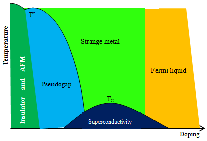Figure 1. (colour online): The transition phase diagram of high temperature superconducting cuprates showing the various phases at various temperatures and doping levels

2. Modeling

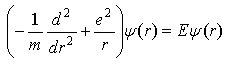
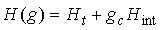
Modeling is an attempt to mimic reality in a controlled scenario. In physics, a model can be conceived as a simple and well understand phenomenon or system designed to represent and explain a complex and not well understand phenomenon or system. Therefore the model should possess the domineering properties of the phenomenon or system it is supposed to represent. The two main components of chaotic tendency are the ideas that (1) that small changes in the initial conditions can lead to widely diverging outcomes and (2) no matter how complex a system may be, it rely upon an underlying order [31, 32]. It is stated above that the transition from normal to superconducting state is nonlinear hence a chaotic tendency. Since doping influence the electronic composition of the parent materials, then we need to first identify the material specifics in which changes in their initial conditions in the normal state gives rise to the transition phase diagram hence superconductivity [25, 33-37]. In their structural analysis of the high T_C superconducting cuprates, Villars and Philips observed that there are three ‘golden coordinates’ that drives the superconductivity namely orbital radii, valence election and electronegativity [34]. This has been recently extended to the valence electrons, atomic number, formula weight and other factors [35]. Their study is an attempt to generalize the Matthias approach [36, 37] of using periodic table and material specifics to predict superconducting materials and their transition temperatures which was successful for the conventional superconductors to other families of superconductors. While there have been no experiment to confirm or refute their predictions, it is my thinking that their approach may help to understand the high T_C superconducting cuprates. Therefore in the study here, the changes in the aforementioned material specifics will be modelled as influencing the doping which in turn triggers the phase diagram.

Classically, the motion of a body can be described by its dynamic variables such as its velocity, mass and time. However, the Heisenberg principle restricts such description in quantum mechanics to variables such as momentum p, position r and time t (not often). This restriction makes it necessary to re-express the total energy of a quantum physical system in terms of p, r, and t only. This can be expressed mathematically by the conventional quantum mechanical equation in relative coordinates and reduced mass for two electrons in singlet coupling as

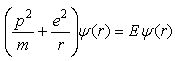(1a)

where m is the mass of the electrons.

The replacement of the classical variables in Eq. (1) by their corresponding quantum mechanical operators will result in a second order differential equation Hamiltonian for two repelling electrons and therefore a nonlinear system:

(1b)

By second quantization of this Hamiltonian [38, 39], we obtain the Hamiltonian with the creation and annihilation operators. This could be the Hubbard model and its various extensions [40, 41] or its strong coupling limit known as the t-J model and its various extensions [38, 42, 43]. The general form of these models can be expressed as [24]:

(2)

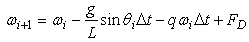
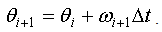
where is the kinetic part and is the interaction part which determine the quantum fluctuation with the denoting the tuning parameter. The QCT occurs when reaches a value denoted by that can trigger the QCP.

The classic system to describe nonlinear physical systems is the nonlinear pendulum and the equation of its dynamics is [28]

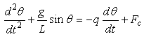(3)

where

g is acceleration due to gravity,

L is the length of string,

is the velocity dependent damping force and

F_c is the sinusoidal driving force that captures the initial conditions of the material specifics such as orbital radii r, electronegativity valence electron count N, atomic number Z and formula weight Fw [35], that is,

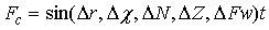(4)

In the Hamiltonian representation of the high-T_C superconducting cuprates in (2), the effects of both the damping force and the driving force are captured in its interaction part. In the modelling here, we assume the system with only damping force as the undoped case while the inclusion of the driving force is the doped case. Therefore the value of F_c hence the changes in the initial conditions will determine the phase transition, with F_c = 0 being the system with no changes in the initial conditions. Further, we start from the basic assumption of the Hubbard model that the undoped material is antiferromagnetic (AFM) at low temperature and that doping eradicates the antiferomagnetism hence the material becomes superconductive [40]. In the case of the t-J model, we start with the basic assumption that the undoped material is AFM at low temperature as in Hubbard model while the doped material of the t-J model is assumed to possess short range AFM and SC [41].

Comparing (2) and (3), the first part of both the LHS and RHS of (3) represents the kinetic part of (2) and the remaining part is its interaction part. Therefore, the dynamics of the phase diagram of the superconducting cuprates is simulated with (3) by representing the temperature with theta and the doping with time. This is achieved by using a modified Euler’s Method for solving differential equation, the Euler-Cromer Method [28] to solve (3) after breaking it down to two first order systems:

(5)

with

(6)

Equations (5) and (6) are then coded using Python to obtain the solution of the (3).

3. Presentation and Discussion of Results

The starting point of the numerical results is to consider the normal state conditions wherein F_c = 0. As depicted in Figure 2, the output is a normal damped sinusoidal curve which will be considered as the insulator and AFM state of the phase diagram as shown in Figure 1. Introducing changes in the initial conditions implies that F_c > 0 resulting in a transient waveform depicted by the red box followed by a normal sinusoidal curve in Figure 3. If we compare Figures 1 and 3, then the transient waveform in Figure 3 is the pseudogap in Figure 1 while the normal sinusoidal curve is the superconducting state. This scenario of changes from F_c = 0.01 (Figure 3a) to F_c = 0.02 (Figure 3b) is equivalent to slight enhancement of the doping as we increase the amount of the material specifics. In both cases, there is still a small region of damped sinusoidal curve, followed by a pseudogap phase and then a superconducting phase. However, it is easy to see that as we increase from F_c = 0.01 (Figure 3a) to F_c = 0.02 (Figure 3b), both the regions of damped curve and pseudogap curves decrease while that of the superconducting region increases. Further, the portion of the visualized phase diagram where the QCP indicating the change from the pseudogap to the superconducting curves is likely to be, is from time = 95 – 146 when F_c = 0.01 and from time = 64 – 113 when F_c = 0.02. The common feature to both visualized phase diagrams is that the change from the AFM region to the peudogap region was abrupt while that of the pseudogap to the superconducting region is slow. This is a visualization of the well known results of the time-resolved reflectivity measurements at different temperatures which shown that a fast-changing, negative signal sets in below T* that is distinct from the slow-changing, positive signal at the onset of T_C [21]. This is often considered as the signature for the different nature of both pseudogap and superconducting phases [15, 16, 21]. Increasing the material specifics from this point (starting from F_c = 0.03), the visaulized phase diagram now starts from the pseudogap region followed by a more enhanced superconducting phase and the region to find the change from pseodogap to superconducting region decreases where for F_c = 0.03 (Figure 4a) it now lies from time = 62 – 97 and for F_c = 0.27 (Figure 4b) it lies from time = 49 – 96. Also, the pseudogap curve seems to be changing gradually into a sinusordal-like curve as the driving force is increased from F_c = 0.03 to F_c = 0.27. Logical prediction expects both the pseudogap region and the region of the transition from the pseudogap transient waveform to the superconducting region to shrink further and even probably be absorbed into the superconducting phase as we increase the F_c beyond F_c = 0.27. But as clearly shown in Figures 5a and 5b, the pseudogap changes into a damped-like curve whose size increases as the driving force is increased from F_c = 0.28 to F_c = 0.29. Similarly, the region where the QCP lies is also increased from time = 49 – 94 for F_c = 0.28 to time = 79 – 111 for F_c = 0.29. This means the new damped-like curve which we likened to the strange metal region in Figure 1 now increases rapidly at the expense of the superconducting region in the optimal doping level. This is in line with the experimental observation of the change in the quasiparticle decay rate and the sign of the photoinduced change in reflectivity measurement in BSCCO system superconductors precisely at optimal doping [44]. Thus this is an indication that the onset of quantum fluctuation responsible for the pseudogap region at T* are quenced around the optimal doped region. This agrees with the experimental observation that the pseudogap state only sets in when the hole doping of the cuprate is neither too low nor too high [20]. The reason why the pseudogap curve does not return to exactly to the waveform of the normal state after the quenching of the quantum fluctuations that caused it may be due to the nonadiabtic nature of this quantum criticality [24, 45]. Thus the inference is that in this optimal doped level, the pseudogap has crossed into the strange metal regime in agreement with studies [22, 44, 46] which observed the existence of an additional hidden QCP around the optimal doping. This may also be related to the experimental study of the electronic Raman scattering in overdoped (Y,Ca)Ba₂Cu₃O_y wherein it is observed that there is electronic crossover due to the collapse of the pseudogap [46]. This has been visualized here as the values beyond the optimum doping, that is, F_c > 0.29, which is choatic and hence non-superconducting state as shown in Figure 6 for F_c = 0.30.

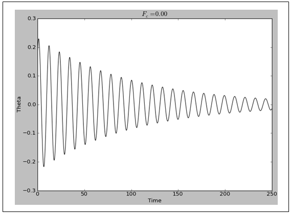Figure 2. The damped sinusoidal curves of the normal state, that is, when there are no changes in the initial conditions so that FC = 0

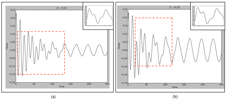Figure 3. (colour online). The damped curves, chaotic curve and sinusoidal curve when there are changes in the initial conditions so that Fc > 0 for (a) Fc = 0.01 and Fc = 0.02. In both cases, the red dash line indicates the pseudogap phase while the inserts are the regions wherein the quantum critical point possibly lies (a) from (time = 95 – 146) and (b) from (time = 64 – 113)

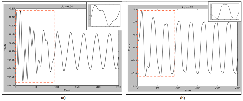Figure 4. (colour online). The damped curves, chaotic curve and sinusoidal curve when there are changes in the initial conditions so that Fc > 0 for (a) FC = 0.03 and Fc = 0.27. In both cases, the red dash line indicates the pseudogap phase while the inserts are the regions wherein the quantum critical point possibly lies (a) from (time = 62 – 97) and (b) from (time = 49 – 96)

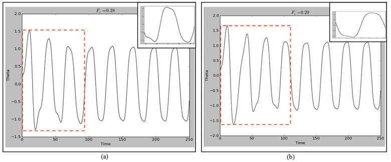Figure 5. (colour online). The chaotic curve and sinusoidal curve when there are changes in the initial conditions so that (a) FC = 0.27 and FC = 0.28. In both cases, the red dash line indicates probably the strange metal region while the inserts are the regions wherein the quantum critical point possibly lies (a) from (time = 49 – 94) and (b) from (time = 78 – 111)

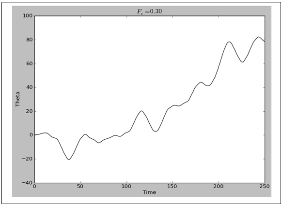Figure 6. The nonsinusoidal curves of the nonsuperconducting state, that is, when there are changes in the initial conditions beyond optimum doping so that for Fc = 0.30

4. Conclusions

A basic Hamiltonian to account for the phase diagram of the high T_C superconducting cuprates has been modelled as a nonlinear system. It turns out that the visualized phase diagram fairly captures the essential features of phase diagram of the high T_C superconducting cuprates. At small values of the driving force which represents the material specifics that influence the doping, there is abrupt change from the normal damped curve representing the Mott insulator and antiferomagnetic state to a transient waveform which depicts the pseudogap region. This abrupt change is a signature of avoided crossing [24] and it indicates the presence of a QCP and therefore the pseudogap is a manifestation of QPT due to quantum fluctuations. Now as the driving force is increased, there is a slow change from the pseudogap transient curve into a sinusoidal curve. This is likened to change from the pseudogap region into the superconducting phase. One is tempted to assume that this slow change is a signature of smooth crossing so that there is no QCP between the pseudogap and the superconducting state. This would have supported the school of thought that the same carriers interaction mechanism is responsible for both the pseudogap and the superconducting regions of the phase diagram of the high T_C superconducting cuprates. This expectation is enhanced by an observable trend of a decreasing pseudogap curve that seems to be gradually changing into a sinusoidal-like form and more slowly crossing into an expanding superconducting curve as the driving force is increased from F_c = 0.03 to F_c = 0.27. It is observed, however, that as the driving force is increased to F_c = 0.28, the pseudogap transient curve abruptly changes into a damped-like curve but still maintain its smooth change into the sinusoidal curve. It is pertinent to point out that this behaviour have been observed in superconductivity fluctuation measurement of high-T_C cuprate wherein it was observed for the hole doped LSCO, the universality class was found to change twice as a function of doping, starting from the 2D-XY, changing to the 3D XY and another 2D “unknown” behaviour [22]. Therefore we assume here that at around the optimal doping the pseudogap phase has transit into a different phase (likely the strange metal region) from the superconducting phase but may be related to the normal state as both have damp-like waveforms. Thus the pseudogap all along has been a competing phase with the superconducting phase and not its precursor [15, 16, 20, 22, 44]. It follows then that if we are to critically study the phase diagram of the high T_C superconducting cuprates using the visualized phase diagram as our guide, then we have to first confirm the existence of the three quantum critical points and these are the QPT from the Mott insulator and AFM phase to the pseudogap at slight doping, the QPT from the pseudogap to the superconducting phase at minimum doping and the hidden QPT of the pseudogap probably into the strange metal region around optimal doping.

The fair representation of the often considered complex phase diagram of the superconducting cuprates by a simple nonlinear dynamic equation has also provided a guide to the possible Hamiltonian as well as the possible theory for this class of superconducting materials. The formulation should be such that the quantum fluctuations to kick start the pseudogap region at slight doping will competes with the one responsible for the superconductivity at minimum doping until it will be quenched around the optimal doping. The emerging state from the collapsed pseudogap state is nonadiabatically related to the normal state as well as the non-Fermi liquid state.

ACKNOWLEDGEMENTS

I acknowledge that part of this work was done at the Max Planck Institute for Physics of Complex System, Dresden, Germany. This work is partially funded by ICBR.