John Kulick
University of Connecticut, Connecticut USA
Correspondence to: John Kulick , University of Connecticut, Connecticut USA.
| Email: |  |
Copyright © 2014 Scientific & Academic Publishing. All Rights Reserved.
Abstract
This is the first of 4 papers describing a Unified Field Theory based on a Multidimensional Geometric Expansion of Spacetime. Assumptions and properties of model – 1. Spacetime is defined by field based or structural relationships of distance and time. 2. The expansion of Space does not stop at the boundary of galaxies, but incrementally within the atom itself, thereby yielding the probabilistic properties associated with Quantum Mechanics. 3. The volume of Spacetime, or object, S, when viewed from an Absolute or “Eye of God” perspective outside the expansion, varies to the square of the Cosmological measure of time. Double the Age of the Universe and the volume increases 4 times. 4. Since “absolute” density decreases over time, the effect of gravity diminishing over time. (Effect of gravity varies by T^(-4/3) where T = Historical Location/ Age of Universe). 5. A local observer within “Observable Space” would not perceive any change in local measures of distance and intervals of time since all local clocks and local rulers proportionally change at the same rate. 6. Since all clock rates were faster in the past, cumulative measures of time experienced locally would actually be greater than would be expected when compared to Cosmological measures of time. 7. Stars would evolve more quickly than presently assumed, potentially resolving the issue in which some stars in Globular Clusters are determined to be older than the Universe. (This issue is not as resolved as many are inclined to believe). Two geometrically related and independent measures of time are established, local and Absolute, (also called Historical or Cosmological). 8. Accelerative fields associated with charge and gravity are predicted field relationships, which unites the two forces based on a dynamic multidimensional geometry. The succeeding papers are based on an expansion of the proposed model, wherein Observable Space is expanding within a moving and similarly expanding Unobserved Space.
Keywords:
Unified Field Theory, Expansion of Spacetime, Two Dimensions of Time, Gravity Decreases over Cosmological Time, Age Problem of Stars Older than Universe
Cite this paper: John Kulick , A Multidimensional Geometric Expansion of Spacetime, International Journal of Theoretical and Mathematical Physics, Vol. 4 No. 2, 2014, pp. 17-36. doi: 10.5923/j.ijtmp.20140402.01.
1. An Alternative Model for the Expanding Universe
Astronomy books describing the expansion of the Universe often use an illustration of a balloon with pennies or buttons stuck onto the surface of an expanding balloon. (“Gravitation” by Misner, Thorne and Wheeler Pg 719 Figure 27.2 23 printing in 2000 [1]). The pennies represent galaxies and the expanding balloon represents the expansion of Spacetime. The expansion stops at the boundary of gravitationally bound galaxies. Bradley W. Carroll and Dale A Ostlie in their book “An Introduction to Modern Astrophysics” pg 1116 copyright 1996 [2]), write the following about the expanding Universe. “It is important to realize that although the universe is expanding, there is no compelling evidence that the constants that govern the fundamental laws of physics, (such as Newton’s gravitational constant, G) were once different from their present values. Thus the sizes of atoms, planetary systems, and galaxies have not changed because of the expansion of space (although the latter two may have certainly gone through evolutionary changes).” (The italic is in the original text)What if galaxies, planetary systems and even atoms expanded with the expansion of Spacetime? Initially such a consideration sounds preposterous. If atoms and Solar systems expanded, wouldn’t they become unstable and fly apart? Local rulers would keep their proportional measure, but what about clocks and clock rates? As established in the book about General Relativity previously referenced, “Gravitation”, time is a part of the structure of spacetime. If Spacetime expanded wouldn’t the very structure of spacetime be destroyed by such an expansion? The questions are numerous and fundamental. In the course of this paper these questions will be addressed. Additionally, there will be rewards for considering such a model. For example, Dark Matter and Dark Energy apparently are not needed to explain the motion and location of galaxies and the forces of Nature become unified.
2. Theory Published in 4 Papers
This paper is the first of four with each building upon the next. The topics described in each paper are 1. The Expansion of Observable Space. The relationships associated with a geometric expansion of Observable Space are defined.2. Expanding the Expansion. The relationships associated with the Motion of Observable Space within an Expanding Unobserved Space are defined.3. Unified Space. The integration of the effects from Observable Space and Unobserved Space are combined and described from an Absolute and local perspective.4. An Intrinsic Extra dimensional deceleration is predicted within Unified Space, which is applied to Cosmological structures such as spiral galaxies and the location of galaxies over time.
3. Heading, Figure and Equation Designations
3.1. Headings
The first number in the headings refers topic’s sequential location in the paper. The second number describes the sequential sub topics location within the basic topic. Minor additions to a topic or Subtopic will not be numbered but written in bold.
3.2. Figures
The Figures will be labelled by sequential location in the paper.
3.3. Equations
Equations are labelled first by topic or chapter location, than sequentially within the topic, within a set of parenthesis.A second set of equation numbers may be included after the primary location number. This second set of numbers is included to allow the reader to find the original derivation of the formula.Later, in successive papers, a numeral will be added to the front of the equation designation to know in which paper the relationships were derived. For example, (II.2,3) refers to an equation derived in the Second Paper.
4. Acronyms of Models
Since the presently accepted Cosmological model stops the expansion at Galaxies, it will be referred as the Limited Expansion Model (LEM), or the “Dark Model” since the current model also requires that most of the Universe be composed of Dark Matter and Dark Energy.Since the proposed model is based on a geometrically defined expansion of Spacetime, it will be referred to as the Geometric Expansion Model (GEM). Adding the Extra dimensional aspect of the model to the name would be a bit long and mess up the nice Acronym. Actually a gem like description of the dynamic structure of Space is a very good representation of the proposed model.
5. Graphical Comparison of Models
The following figures compare the presently accepted expansion model to the proposed model using common balloon analogy.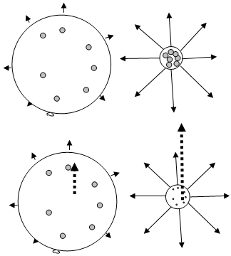 | Figure 1. Balloon Analogy comparing Two Models |
The upper two balloons represent the present Limited Expansion Model (LEM). The lower two balloons represents the Geometric Expansion Model, GEM. The larger balloons represent a present description of the Universe and the smaller circles represents the Universe when it is younger. The small circles within the balloons represent galaxies. The arrows around the balloons represent the rate of expansion. The dashed arrow for the GEM represents the velocity of an Unobserved Space moving past or through the Observable Universe. One obvious difference in the models is the size of galaxies over time; in the early Universe the LEM has all the fixed sized galaxies on top of each other, whereas the GEM has all the galaxies converging on to themselves with an initial separation between galaxies. Both models share the same belief that it is the expansion of spacetime that is carrying the galaxies. Galaxies are not actually moving with respect to the structure of Observable space, but are being carried by the expansion of spacetime. (This description will be modified when the effects of the expansion along the Unobserved dimension are incorporated into the model).
6. Outline – Expansion of Observable Space
1. An Alternative Model for the Expanding Universe2. Theory published in 4 Papers3. Heading, Figure and Equation Designations3.1. Headings3.2. Figures3.3. Formulas4. Acronyms of Models5. Graphical Comparison of Models6. Outline – Expansion of Observable Space7. Expansion Models of Others8. Absolute and Relative8.1. Perspectives8.2. Absolute Formulas describing Nature9. Definitions and Notation10. The Geometry of Expanding Observable Space – Derivation of Basic Formulas11. The Ratios of Time12. Cosmological “k”13. Intervals of Time in an Expanding Spacetime Field14. Time and Structure15. Do Relative Measures of Intervals of Time stay the same?16. The Boundary or Edge of Space16.1. Boundary within Atom16.2. Crinkled Boundary becomes 3-D “foam”16.3. Separation between Observable Space and Unobserved Space16.4. Growing by Unfolding Bits of Spacetime17. The Kinematics of Expansion17.1. The balloon analogy17.2. Effect of Bits of Spacetime on Velocity17.3. Object Moving Through Expanding Spatial Fabric17.4. How should Velocity Change over Time?17.5. Assumption - The Geometry of Energy Loss17.6. Generalizing the Equations to Acceleration17.7. Whoa! General Relativity defines acceleration of Gravity17.8. Change in distance 17.9. Fundamental Properties are the result of a Geometric Expansion of Space18. Intervals of Relative and Absolute Time in an Expanding Spacetime field18.1. Intervals of Time and the Light Clock18.2. Intervals of Time and Momentum18.3. Intervals of Time and the Pendulum18.4. Intervals of Time and Kepler’s 3rd Law19. Two Dimensions of Time19.1. Absolute, Cosmological or Historical Measure of Time19.2. Experiential Time in Observable Space20. First Testable Prediction of Model20.1. Age of Stars20.2. Papers about Stars Older than the Universe21. Forces, Spatial and Inertial21.1. How Spatial Forces change over Time21.2. How Inertial Forces change over Time21.3. Orbital Stability21.4. Another Benefit – A Unified Field Theory22. Energy22.1. Work22.2. Potential Energy – Inverse square Laws22.3. Potential Energy – Constant Field22.4. Elastic Potential Energy22.5. Kinetic Energy22.6. “Rest” Energy of Mass23. Issues with the Energy of a Photon23.1. Fundamental Problems with the Cosmological Red Shift for the LEM 23.2. Fundamental Issue for the GEM23.3. A Photon’s Energy23.4. f- Energy variation by frequency23.5. c/λ – Energy variation by c and λ23.6. Check for Proportional Change in Energy23.7. Predicting a Cosmological Red Shift – with issues23.8. “Old Photons” – More issues24. Special and General Relativity24.1. Special Relativity24.2. General Relativity25. Cosmological Measures of Distance and Time25.1. Variation from the LEM25.2. Something “off” with the LEM and Expansion26. Look Back Distance and Look Back Time27. Problem for GEM. No Expansion!28. More issues for GEM – Cosmological Time Dilation28.1. Cosmological Time Dilation is observed28.2. Except with Quasars28.3. Derivation of Dilated Intervals28.4. The Problem –Dilation is canceled by faster Clocks29. Dimensions of Space29.1. Location of a Point29.2. Physical Properties and Dimensions29.3. Dimension of Absolute Time and Physical Properties29.4. Dimension of Time and describing a Points Location29.5. Criteria for Dimensions29.6. The three physical dimensions of spatial space29.7. Distance Dimensions for Gravity and Charge29.8. More Dimensions - Spin30. Summary30.1. Issues with GEM30.2. Benefits of GEM30.3. Predictions of GEM31. The Snowflake Universe32. Formula of Expanding Observable Space33. Expanding the Expansion
7. Expansion Models of Others
There are two individuals that this author is aware of that also propose an expansion based model that does not stop at the boundary of galaxies, John Hunter of England and C. Johan Masreliez of the USA. None of us were aware of each other’s work and we each were independently inspired to consider an expansion model. John Hunters’ work can be found by an Internet search underwww.rescalingsymmetry.com [3] John Masreliez’s work can be found under a search using the terms “expanding spacetime theory” [4], or a peer reviewed paper at [5] For those familiar with General Relativity, the relationships derived by Masreliez will be of particular interest to review.Both Hunter’s and Masreliez’s work is based on using relative measures of distance and time, whereas the proposed relationships are derived using a constant or absolute measure of time. I presented a paper that proved the models were geometrically transformable one to the other at a conference for the American Physical Society in April of 2005 when just the expansion of Observable space is considered. (Reference not included since link to paper titled “Hypothetical geometric expansion with two dimensions of time” could not be found within APS archives).
8. Absolute and Relative
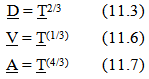
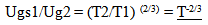
The following figures will help establish some of the concepts and terminology of the model which are important for understanding the formulas generated.Using a ruler established at T1, a pizza is measured to be 1 Unit of length long. At T2, using a local relative ruler that has expanded with the structure of spacetime, the pizza is still measured to be 1 unit long since the ruler has expanded with the pizza. From the “Eye of God” perspective it can be seen that when using an “absolute” ruler established at T1, that the pizza is now 1 and 2/3 longer.
8.1. Perspectives
The “Eye of God” perspective represents a vantage point from which the expansion can be observed or described. The necessity for this perspective results because a local observer would not be able to see or easily measure the expansion with locally expanding rulers and clocks. This “Absolute” perspective establishes a framework upon which the change in relative measures can be described. Locally all the fundamental relationships will always be preserved, such as the relationships of Special Relativity and General Relativity. However, from the Absolute perspective, the variation of these relationships over time can be described.
8.2. Absolute Formulas Describing Nature
The description and development of the model will be done using the “Absolute Perspective”. While fundamental properties of nature will be changing over “Absolute time”, what will be shown is that from a local perspective, the fundamental relationships of nature are essentially the same over time. The laws of nature are built upon an expanding framework.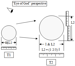 | Figure 2. Absolute and Relative Ruler |
9. Definitions and Notation
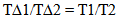
The proceeding graph affords a reference for some of the basic terms and notation used in this work. 1. Capital letters refer to an Absolute or “Eye of God” measure of an object based on a ruler or clock that is “fixed”. 2. Lower case letters refer to a local measurement using a local ruler or local clock that is expanding with the fabric of spacetime. 3. A “1” or “2” after a letter designates an earlier and later measure respectively, such as T1 and T2.4. Absolute measures of time are also called Historical or Cosmological Time since this measure of time defines a point’s location relative to the beginning of time.5. An “o” after a term designates a present measure. For example, “To” is used to represent the present Age of the Universe.6. A reference measure of time or distance is established at some particularly point in time, usually the present, To, which is then used to describe the variation in measures in the past.7. “S” refers to a volume of Spacetime, including the matter within that Spacetime.8. “==” The double equal sign represents a proportional relationship that is geometrically based.9. Ratios of similar physical parameters, such as time or distance that are compared over historical periods of time will be expressed in a short hand notion using an underline. For example T1/T2 = T; D1/D2 = D. Note that earlier measures are to be placed over later measures.10. The word “Space”, when capitalized, has the same physical meaning of the usually hyphenated word “space-time”. Time is a part of the structure of Space.
10. The Geometry of Expanding Observable Space Derivation of Basic Formulas
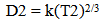
The geometry of Expanding Observable Space is defined by a very specific relationship. A volume of Spacetime varies to the Square of the Cosmological Time Elapsed. Double the age of the Universe and the volume of Spacetime, and all the objects within it, will increase 4 times.  | (10.1) |
This variation in volume is based on an Absolute or “Eye of God” perspective outside of the Expansion. Based on local or relative measures there is no locally observed variation in the measures of distance or volume. Even local measures of time show no local variation, which will be discussed later. Since the volume of anything is some constant times a length measure of that object cubed, | (10.2) |
(The inverse of the constant k is used to make the form of the following formulas easier.)Equating equations 1 and 2, | (10.3) |
Which results in,  | (10.4) |
(Looks like Kepler’s 3rd Law, coincidence?)Which leads to  | (10.5) |
The following figure illustrates the variation in an objects’ linear measure with the passage of absolute or Cosmological time.
11. The Ratios of Time
The geometry of the model allows comparisons to be made over time. At one point in time, T1, the volume and distance measures are a certain size, and at T2 the volume and distance measures are another. Dividing the two relationships by each other allows the elimination of the constant k.  | (11.1) |
 | (11.2) |
Divide one equation by the other results in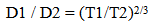 | (11.3) |
The first derivative with respect to absolute time of the distance measure described in equation 5 yields a velocity term and the second derivative of the distance measure yields an accelerative relationship.  | (11.4) |
 | (11.5) |
Repeating the ratio type derivation for acceleration and velocity.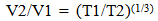 | (11.6) |
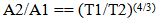 | (11.7) |
At this point, the ratios of time correspond to relationships between two points that are being expanded according to the proposed geometry. They will take on a more significant meaning later in the development of the model.Using the Notation standard described earlier the Ratios of Time can be expressed as follows in Table 1.The Ratios of TimeTable 1. The Ratios of Time
 |
| |
|
 | Figure 3. Comparing size of object over Cosmological Time |
12. Cosmological “k”
First, a point of clarification. “k” is an overworked symbol, found in thermodynamics, the spring constant or as any generalized constant. More conventional cosmological models associate “k” with a scale factor. Its’ value also correlates to the curvature associated with spacetime. The proposed models use of “k” is not to be confused with these pre-existing uses. If the Observable Universe begins when T1 = 0, then the simplest assumption would be that the distance between points when T1 = 0 would also be 0. This ignores the possibility of an initial offset between points when the universe began. This assumption would also result in the present radial size of the Universe, (from two points being initially together, to their observed present separation) to be defined as… | (12.1) |
 | (12.2) |
If it is assumed that the speed of light defines the relationship between points with respect to distance and time, (an assumption that will be justified later in the development of the model), then the size of the observable Universe is equal to the speed of light times the age of the Universe. | (12.3) |
This allows k to be expressed in terms of the radial size of the Universe and the present Age of the Universe, To. | (12.4) |
k is equal to the speed of light times the cube root of the age of the Universe.
13. Intervals of Time in an Expanding Spacetime Field
It is obvious that proportional measures of distance keep their proportional relationship since everything is proportionally expanding equally. However, what about intervals of time? For example, consider a pendulum. At T1 it has a given length while at T2 it is longer. Since the period increases as the length of the pendulum increases, one would expect that from an absolute perspective that intervals of relative time would slow over the passage of historical time.
14. Time and Structure
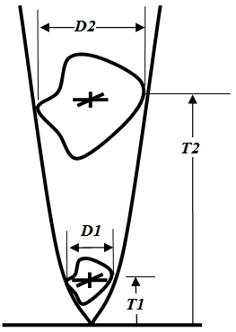
Time is a part of the fabric of Space. If we expand Space, time must be affected. This is illustrated in the following figure which represents a proportional matrix like expansion of Spacetime.Each point at every intersection on the left side of the above figure represents a spatial separation of 300,000,000 meters, with a relative temporal separation of one second between each neighbouring corner or intersection. This one second temporal separation is the time it takes for light to transverse the distance either laterally or horizontally to a nearby intersection point. 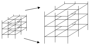 | Figure 4. Preserving relative measures in spacetime |
After expansion, according to the proposed model, each point in the matrix would still be separated by a relative interval of distance of 300,000,000 meters. After expansion would there still be a relative temporal separation between points of one second of time? In order for the model to be correct, expanding the structure of spacetime requires all relative measures of distance and time between points to stay the same, or be locally invariant.
15. Do Relative Measures of Intervals of Time Stay the Same?
This variation in the measure of an interval of time raises some issues. Would intervals of time maintain their local proportional measure in all physical relationships? For example, would an interval of time described by a light clock change at the same rate that an interval of time described by a pendulum, or an orbiting system, vibrating objects, or resonant electrical relationships? This issue will be addressed after some of the dynamic and physical consequences of the model are considered.
16. The Boundary or Edge of Space
Often the edge of space is assumed to be a far off distant location. For the proposed GEM this perception would be wrong. The past, as observed when we look into outer space, defines the structure of the Universe as it was in the past. The edge of space exists in the present and it is where we are now.
16.1. Boundary Observed within the Atom
The “Boundary” is a part of space itself. The observation of this boundary is found within the atom itself.
16.2. Crinkled Boundary becomes 3D “Foam”
If a surface like construction of the boundary of space is to be visualized within three-dimensional space, it would be a very “crinkled” surface that acts like a three dimensional volume. This is similar to the fractal based geometry in which a crinkled up piece of paper is dimensionally described as containing 2.5 dimensions. If the paper were sufficiently and properly crinkled, the dimensional representation would increase above 2.5 dimensions and “fill” a 3 dimensional space. The “Quantum Foam”Since this crinkled surface is changing, it is this process that provides the physical explanation for what is called the “quantum foam”.
16.3. Separation between Observable Space and Unobserved Space
This “surface” would establish a boundary between our observable space, and an extra dimensional space outside our Observable Universe called “Unobserved Space. The expansion of this boundary would behave like an unfolding process. The relationship between Unobserved Space and Observable Space will be developed in succeeding papers.
16.4. Growing by Unfolding Bits of Spacetime
The expansion of Space along this boundary is proposed to occur incrementally; a subatomic volume of spacetime integrates itself upon the existing fabric of reality a bit at a time. (Called ?) The process can be visualized as a kind of unfolding since the growth comes from within Space, and all the objects within Space.
17. The Kinematics of Expansion
Expansion takes energy. Since this expansion is occurring everywhere, than all things are experiencing a loss of energy.
17.1. The Balloon Analogy
Consider an expanding balloon. The surface tension in the balloon decreases, which allows the balloon to expand. There is a corresponding drop in pressure, and a drop in the velocity of the molecules and thus a drop in the temperature and energy contained in the balloon. Similarly there should be a kinematic loss of any object in motion as the boundary of Observable Space expands.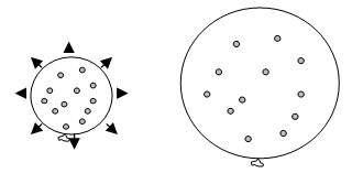 | Figure 5. Expansion and Kinetic Loss |
17.2. Effect of Bits of Spacetime on Velocity
The incremental “voids” or “pieces” of spacetime that are integrating themselves upon the existing structure of reality interact with objects as they move through them. The “retreat” of Space or the fabric of Space due to expansion would mean that any object passing through such a sub atomic scaled void, would have to travel further, and absorb the void, resulting in a slowing of the objects motion. Kinetic energy would diminish.
17.3. Object Moving through Expanding Spatial Fabric
The other expectation of the model is that the rate that the velocity diminishes should be proportional to the velocity of the object based on the physical characteristics of the model.If objects in motion are moving through an existing invisible expanding field structure, the faster they move through the expanding field the more of the expansion the objects would have to pass through. The more of the expanding field the object passes through, the more kinetic energy would be “absorbed” by the expansion. Motion actually comes at a cost. This is going to affect the understanding of the Newtonian concept of an object in motion and conservation of momentum. 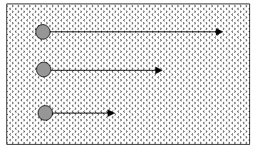 | Figure 6. Voids encountered proportional to speed |
17.4. How should the Velocity Change over Time?
The next question becomes how fast or by what kind of relationship should the proportional reduction in velocity occur? It is proposed that the same geometric relationships that describe the expansion of observable space also describe the geometry of absolute measures of distance, velocity and acceleration associated with an object within this expanding metric.
17.5. Assumption – The Geometry of Energy Loss
If an object in observable space is moving away from a point in Observable space, as seen from the “Eye of God” perspective, then the proportional change in the velocity of the object moving in an expanding spacetime field is defined by the same Geometric Expansion Formulas derived for the variation in the measures associated with a volume of Space. For example, if the present rate of expansion is 1/2 of what it was at some point in the past, the velocity of an object traveling through the expanding space time field during that time, if uninfluenced by other factors, would also be reduced by a half.
17.6. Generalizing the Equations to Acceleration
Since the velocity of moving objects is changing at a specific geometrically defined rate, the same effect would be realized with acceleration. The proposed formulas describing the effect on objects moving in an expanding spacetime metric or field are…Velocity of object at T1/ Velocity of object at Acceleration of object at T1/Acceleration at
17.7. Whoa! General Relativity Defines the Acceleration of Gravity
Those familiar with General Relativity are sure to have some reservations to any model that is now ascribing accelerative fields to be the result of expansion, as opposed to the assumption of General Relatively in which it is the interaction of matter causing a curvature of space, which is what produces the accelerative field. Be patient, it will be shown that none of the relationships associated with the use of general relativity to local gravitational relationships has changed. Also, those familiar with General Relativity may see that the underlying philosophy of describing relationships based on intervals of distance and time is a shared perspective used in both models.
17.8. Change in Distance
If it is assumed that the interval of time over which distances, or time elapsed traveled of a moving object are small in comparison to the Age of the Universe. Distance traveled of object, ∆D1 at T1 / Distance measure of object, ∆D2 at
17.9. Fundamental Properties are the Result of a Geometric Expansion of Space
This assumption with respect to a more generalized use of the Ratio of Times formulas to include objects moving in an expanding spacetime field, and not just to describe the rate of expansion, will be shown to define a formal structure to Space. Fundamental properties of Space are being established, such as Conservation of Momentum and Conservation of Energy and the Inverse square laws associated with gravity and charge are all being predicted based on an expansion based geometry.
18. Intervals of Relative and Absolute Time in an Expanding Spacetime Field
It has been proposed that objects that are moving in an Expanding Spacetime field change their velocity and acceleration according to the Ratio of Times formulas. This would have a dramatic effect on the measure of time. This poses a rather interesting test for the model. The measure of local or relative measures of time must be preserved or measured to be invariant, while the proportional change observed from the “Eye of God” perspective must be consistent for essentially all dynamic systems. This stark condition is required if space and time are locally invariant. What is going to be done now is apply the Geometry of expansion to some common relationships in Nature. The “Eye of God” perspective “sees” that everything is changing according to a dynamic geometry, yet locally all measures will appear to be unchanged.Once this is done for time, the relationships will be tested for consistency with other fundamental descriptions of nature including, Momentum, forces, and energy.
18.1. Intervals of Time, and the Light Clock
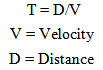
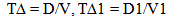
One of the most fundamental relationships in physics or nature is the relationship between distance, time and velocity. Most probably the very first physics problem a student encountered while going to school involved problems that required calculating various algebraic, or more accurately, geometric manipulations of the relationship V = D/T; Velocity = Distance divided by time. The first test will be the application to light.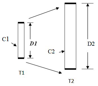 | Figure 7. Absolute Interval of Time and Light Clock |
 | (18.1) |
 | (18.2) |

 | (18.4) |
 | (18.5) |
Sample problem: When the Universe was 1/8th its present age, how much faster was an interval of time defined by a light clock?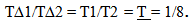 | (18.6) |
As seen from the “Eye of God” perspective, in the past the speed of light was two times as fast and the length of the light clock was 1/4 as long. Note that in order for the model to allow local measures of time to be locally consistent; all clock rates must “tick” 8 times faster in the past. Relative measure of time must maintain their proportional relationship over time, if the model is to be valid.Caveat It is assumed that the local measure for an interval of time is small in relation to the measure of time defining the historical location. This would be what would be presently observed.
18.2. Intervals of Time and Momentum
Now let’s look at the time interval described by an object with momentum with no other forces altering the velocity of the mass, as illustrated in the following figure. The absolute velocity of the object diminishes with the expansion of spacetime. The absolute distance the object has to travel also increases. It may be helpful to associate an “Eye of God” perspective when an absolute measure is referred to since it is only from this “absolute” perspective that these changes are visualized. It is only from the “Eye of God” perspective that the increased distance the object has to travel would be observed using an “absolute” or fixed ruler established at T1.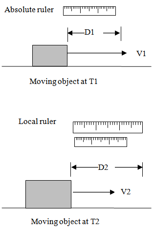 | Figure 8. Conservation of Momentum and Absolute Interval of Time |
The Absolute distance the object travels is now increased with the passage of time, and the absolute velocity diminished with the passage of time. The interval of time described by the object traveling an absolute distance is defined by the objects velocity and the distance the object has to travel.  If a light clock were used to measure the interval of time it took for the object to travel a locally measured distance, the interval of time would be the same at T1 and T2. This example is establishing Newton’s First Law of motion or conservation of momentum.
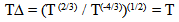
18.3. Intervals of Time and the Pendulum
Now let’s look at a pendulum and a gravitational relationshipThe period of a pendulum is proportional to the square root of the length of the pendulum divided by the accelerative field the pendulum experiences. Applying the predicted relationships for distance and acceleration to the model shows that the interval of time described by the pendulum is the same as the light clock. | (18.9) |
l = length of pendulum, D used in following formulasg = accelerative field pendulum is experiencing(The actual period relationship is a bit more complicated since the amount of deflection is also important but this variation can be ignored since the difference is the same for both.)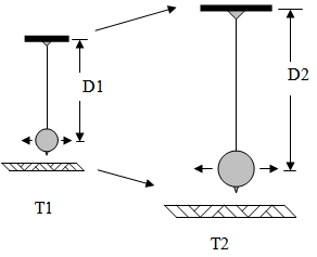 | Figure 9. Absolute interval of time and a Pendulum |
The absolute measures of Distance and the acceleration experienced by the Pendulum are described by… Substituting these values for the period at T1 and T2 to describe intervals of absolute time results in…
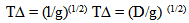 | (18.12) |
 | (18.13) |
 | (18.14) |
 | (18.15) |
Locally intervals of time are measured as invariant but Globally all measures of time are proportionally slowing down at a geometrically defined rate.
18.4. Intervals of Time and Kepler’s 3rd Law
Maintaining the balance in orbital systems is a critical test for the proposed model; without this balance solar systems and atoms could not exist. The orbital intervals of time must also keep their proportional relationships over time. The first check on preserving this balance will be to consider Kepler’s Third law since intervals of time, i.e. the orbital period is expressed simply as a function of a distance measure associated with the elliptical orbit, such as the semi major axis.The figure below illustrates two objects in orbit around each other at two locations in time.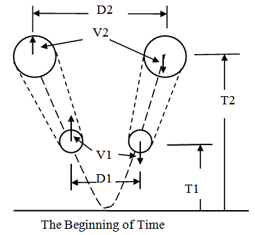 | Figure 10. Absolute Intervals of Time and Kepler’s  Law Law |
== double equal sign, a geometrically proportional relationshipA = semi major axis. (or any geometrically consistent linear measure of the ellipse) Substituting this expression into Kepler’s 3rd Law
 Again the local proportional measures of intervals of time are maintained. Locally all intervals of time appear to remain invariant, but from an absolute perspective, intervals of time are changing.
19. Two Dimensions of Time
Two dimensions of are emerging from this model. They are unique and geometrically related one to the other. Local intervals of time using local clocks are invariant, or unchanging, while the use of a global or “absolute” clock reveals that local measures of intervals of time are changing based on measures of absolute time. The local intervals of time are always the same while from an Eye of God perspective intervals of time are proportionally changing. This relationship is expressed as follows with relative measures symbolized with lower case letters and Absolute measures represented by Capitol letters. 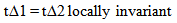 | (19.1) |
 | (19.2) |
When the universe was 1/2 its present age, local clocks ran twice as fast based on an absolute clock.A few terms will help give a more physical meaning to the two dimension of time.
19.1. Absolute, Cosmological or Historical Measure of Time
The absolute, cosmological or historical measure of intervals of time are based on using “absolute” or fixed rate clocks that do not change with the passage of time. Cosmological interval of Time is the measure of absolute intervals of time between points. A common use is to describe a point’s location relative to the beginning of time, or to describe a “look back time”
19.2. Experiential Time in Observable Space
The sequential cumulative measure of local intervals of time using local inertial clocks describes experiential time. This is the time we experience. For now, experiential time will refer to the elapsed time when only the effects of observable space are considered. This measure of time is within the will be modified somewhat when the model. 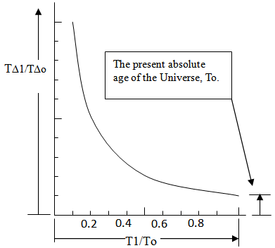 | Figure 11. Relative intervals of time vs. Cosmological Age in Observable Space |
The next graph illustrates the variation in intervals of time over measures of Cosmological time. For example a clock “ticked” 5 times faster when the Universe was 1/5th its present age.Integrating the intervals of time over time yields the measure of experiential time in observable space.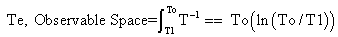 | (19.3) |
20. First Testable Prediction of Model
While all local measures are the same, the cumulative effects over time would not be since the faster clock rates in the past result in a greater measure of experiential time.
20.1. Age of Stars
For example, if a Star was formed when the Universe was 1/2 the present age of the Universe, the total elapsed experiential time the star has evolved to the present would be To(ln2) = .69To. This is greater than what would be assumed using the LEM. Stars should be older than presently assumed.
20.2. Papers about Stars Older than the Universe
The majority of papers which estimated the age of some stars in globular clusters, written since 1982 to 2003 (when I investigated this issue), determined that the stars were older than 14 x 10^9 years. This is older than the current estimated age of the Universe. (13.798±0.037) [7]The adsbs.harvard.edu/abstract/service provided 116 papers written over that time, of which 89 estimated the time for a star to evolve to the great giant stage was greater than 14 x 10^9 years, or 76%. A slight increase in age estimates has to be included to estimates before 1997 because of distance adjustments using the satellite Hipparcos. However, if the time it takes to form the initial stars were included in the age estimates, probably none of the age estimates fall into accordance with the current estimated age of the Universe. (This is somewhat debatable as it could be further argued that some kind of after the fact solution of a hypothetical process would accelerate the initial formation of stars in the early universe.)Using the previous sample problem, it can be seen that a rather significant increase in the evolutionary age of a star is predicted, which would resolve the Age of Stars issue, without hypothetical after the fact solutions.
21. Forces, Spatial and Inertial
Just checking the perseverance of local measures of time does not reveal the extent of the dynamic structure the proposed Geometric Expansion is imposing. The physical effect of expansion on the forces of nature affords another verification of the proposed model. Just as local measures of time have to keep their proportional measure over time, so to must forces. Centrifugal forces must change at the same rate that gravitational and electrostatic forces change, otherwise Solar systems would become unstable, and atoms would fall apart.Since gravity and electrostatic forces are manifested within a spatial field, these forces will be called Spatial forces. (“Spooky forces”). Inertial forces are created when the volume associated with a mass changes either the direction or magnitude of its velocity. (Actually, as will be revealed in the course of the development of the model, spatial forces share the same physical foundation since expansion is imparting an intrinsic motion to all matter and accelerative fields are being created).Spatial Forces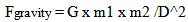 | (21.1) |
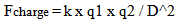 | (21.2) |
From the Absolute perspective, the gravitational constant, Coulombs Constant, and Mass and charge are all constant values, the only the distance between the objects would change over absolute time. This results in… | (21.3) |
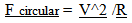
Inertial ForcesThe two inertial forces can be expressed associated with linear and circular motion. | (21.4) |
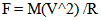 | (21.5) |
The variation in the magnitude of the force, when expressed as a ratio at two differing points in Cosmological time, from an absolute perspective become… | (21.6) |
 | (21.7) |
21.1. How Spatial Forces Change over Time
Spatial Forces diminish by the inverse square of the distances. | (21.8) |
Incorporating the change in absolute distance  Which also is the same rate of change for acceleration predicted by equation…
 This equation is based on the Geometry of Energy Loss assumption. The same relationship that defines how points separate in an expanding spacetime field also establishes the accelerative field an object experiences within the expanding time field. This is a powerful confirmation of the validity of this assumption. The inverse square laws for gravity and charge are being predicted as a result of the structure of an expanding Space.
21.2. How Inertial Forces Change over Time
Inserting how absolute acceleration, velocity and distance change with the passage of time for inertial forces yields… Inertial Forces are diminishing at the same rate that spatial forces are diminishing.
21.3. Orbital Stability
Orbital Stability associated with Atoms and the Solar System is preserved. Actually it is a predicted relationship as a consequence of the proposed Geometric Expansion of Space.
21.4. Another Benefit- A Unified Field theory
The force associated with gravity and that of charge are predicted properties associated with the expansion of Space. This unifies the relationships of gravity with those of charge. All forces respond the same in the proposed expanding Field. | (21.14) |
22. Energy
Do the relationships of Energy keep their proportional relative measures while changing in Absolute measures?
22.1. Work
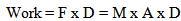 | (22.1) |
 | (22.2) |
22.2. Potential Energy – Inverse Square Laws
The potential energy for an object subject to the inverse square laws are for gravity…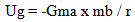 | (22.3) |
Where G ma mb are constant we get | (22.4) |
and for the charge relationship of the electron to the nucleus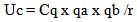 | (22.5) |
Where Coulombs constant is constant, as well as the charges, we get | (22.6) |
Establishing a ratio for two measures of potential energy at two different distances, for objects that experience a force described by the inverse square laws, we get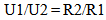 | (22.7) |
Since it is the Absolute Measures that define the potential energy relationship and that it is the absolute distances that vary over measures of absolute time we get | (22.8) |
22.3. Potential Energy – Constant Field Intensity
The potential energy of an object near the surface of the earth is expressed as the mass of the object times the accelerative field (usually understood as the weight of the object), times the high differential available. 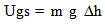 | (22.9) |
Applying the Ratio of time formulas we get
 | (22.10) |
22.4. Elastic Potential Energy
A common example of elastic potential energy is that of a compressed spring. The elastic potential energy is expressed as…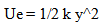 | (22.11) |
where k is a constant of the spring, and y is the distance the spring is stretched.This is an important example since many relationships derive intervals of time using a spring like oscillation to establish intervals of time. For example Resonating crystals, or resonating electric circuits are common in clocks. Initially one may think that this example no longer keeps the necessary proportional equivalence between absolute and relative measures. However this would be to ignore the fact that the atoms of the spring have similarly expanded, which would reduce the amount of potential energy stored within the field relationships of the atom for a given displacement. The magnitude of the force would be reduced proportionally by the proportional expansion of the atom since it is the proportional strain on the atom that produces the force.  | (22.12) |
22.5. Kinetic Energy
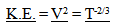 | (22.13) |
Note that this is the same proportional decrease in absolute potential energy that was initially derived for the prediction of how the Kinetic Energy of an object would decrease while traveling through an expanding spacetime field. The pieces of the puzzle keep fitting together.
22.6. “Rest” Energy of Mass
The intrinsic energy of a mass at rest. | (22.14) |
(Formula to be derived in next paper)Assuming that mass is constant, the mass will divide out in a ratio so… | (22.15) |
 | (22.16) |
So far everything is great; all energy relationships are keeping their proportional relationship over time.  | (22.17) |
Things fall apart when the photon is considered.
23. Issues with the Energy of a Photon
Before describing the problem the current model has with respect to the energy of a photon over time, it must be pointed out that this is an issue with the “mainstream” model.
23.1. Fundamental Problems with the Cosmological Red Shift in the LEM
The further away galaxies are observed, the “redder” they appear to be. This Cosmological Red Shift is predicted based on the principles of general relativity, (and the proposed GEM). As a photon travels through expanding spacetime, its energy content is diminished and the wavelength increases. There is a fundamental problem with this prediction of the LEM, as delineated in the following example. In the void of outer space, a gram of matter is converted into radiant energy and beamed to a distant galaxy which has a large mirror that returns the signal. When the light returns, the wavelength of the light has been lengthened and the energy diminished. Convert this energy back into matter and there will no longer be a gram of matter. This indicates three very significant problems. 1. Energy is lost. This violates the principle of conservation of energy. The gram of radiant energy is now less than the gram of matter that was not traveling though outer space. Where did the energy go? The Conservation of Energy law is violated when general relativity is applied in the LEM. 2. Matter and energy no longer equivalent. The relationship, E = mcc defines Energy as equivalent to matter. However, when General Relativity is applied over Cosmological intervals, this is no longer true. A gram of radiant energy does not equal a gram of mass, once the light is traveling through outer space. A fundamental equivalency relationship is being lost.3. Special Relativity predicts that as an object approaches the speed of light, the process of physical change slows down and at the speed of light all physical change would stop. How can a photon traveling at the speed of light change its energy content and wavelength?4. The equivalency of matter and energy is no longer a universal property valid everywhere, but conditional. Equivalency would be maintained within the confines of gravitational bound galaxies).
23.2. Fundamental Issue for the GEM
There also appears to be a problem in the application of the Geometric Expansion model when it comes to describing the Energy of a photon over the passage of time. There is no longer the perfect perseverance of the proportional relationships over time, if matter and energy are to be equivalent over time.
23.3. A Photon’s Energy
The first check for the proposed model is to see if the expression defining the proportional change in the energy content of a photon as defined by the photons frequency, wavelength and the speed of light is consistent.  | (23.1) |
23.4. f - Energy Variation by Frequency
The frequency of the photon establishes a clock like interval, and should vary according to the same principals predicted in dynamic systems. (frequency is inverse to intervals)
23.5. c/λ – Energy Variation by c and λ
 | (23.4) |
Which changes over time in observable space by…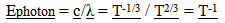 | (23.5) |
23.6. Check for Proportional Change in Energy
 | (23.6) |
The energy of a photon is changing faster than the energy content of other basic systems previously described. For example when the Universe was 1/8th its present age the energy content of mass would have diminished by T-2/3 or 1/4 while the energy content of the photon would have been reduced by 1/8. This is violating the Conservation of Energy observed within Observable Space. Matter and Energy are not equivalent over time. Something is wrong with this model as well.
23.7. Predicting a Cosmological Red Shift – with Issues
The one good aspect to the model is that it is kind of producing a Cosmological red shift. Unfortunately, the energy content varies by T (-1/3) which does not match the expected variation of T (-2/3), The “2/3”rd variation would be expected because the stretch of space varies by the 2/3rds power.
23.8. “Old Photons” – More Issues
The problem is even more pressing when the expected energy of an “old” photon, is observed. The energy the photon loses while traveling through an expanding spacetime field is cancelled by the extra energy the photon starts off with due to the denser electrostatic field the photon was created within the atom. Initial EnergyA photon produced in the past from an atom due to the denser electrostatic field, would have a higher energy value of…  E Photon in produced in Past
 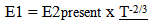 | (23.8) |
Wavelength change with expansionIf the wavelength of the photon changed at the same rate that the expansion of Space occurred, the wavelength would remain the same within observable or local space. A desired relationship that is based on the prediction of Special Relativity in that an object moving at the speed of light cannot physically change. (This would be a change relative to the fabric of observable space, since the relationships of special relativity are observed in our relative observable space).  This same relationship is found when the predicted rate in which energy should be lost from the photon over time, if the variation of the speed of light is ignored.
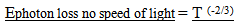 | (23.10) |
Since the energy of a photon is inversely related to its wavelength, this would mean that the expansion of spacetime would cancel out the extra energy the photon started off with. | (23.11) |
This would mean that there would be no cosmological red shift, if the effect of the speed of light on the actual energy content is ignored.Effect of the speed of light slowing over timeOnce the speed of light is incorporated, The prediction is that that the energy content of the photon produced in the past would have to have less energy than it does today. If the wavelength is to be constant, then somehow the speed of light is causing the photon to have a longer wavelength when the photon is created. When the speed of light was faster in the past, a longer wavelength is somehow imparted to the photon. This initially makes no sense and all kinds of gyrations have to be done to resolve it. Most worrisome is the fact that it seems counter intuitive. If the speed of light were greater in the past it makes more sense that the energy content would be greater, even if the photon doesn’t have mass, there is momentum.If the speed of light was greater, then perhaps the wavelength generated would be greater and the energy content would be the same, thereby allowing the rate of energy content to be the same. Unfortunately if this were the case the frequency to energy content of the photon gets thrown off when it is evaluated overtime, resulting in more gyrations dealing with a variable Planks constant. Something is not quite right. It took another 8 years to resolve this issue.
24. Special and General Relativity
A criticism of the proposed model that could be posed is that while Newtonian relationships may be predicted by the model, Newtonian physics is only an approximation derived from the more accurate theoretical models of Special and General Relativity.
24.1. Special Relativity
The relationships of Special Relativity are unaffected in the proposed model. The Lorentz Factor or Gamma is used to define how local measures of the inertia of mass, or the dilation effects of length, or time are changed with respect to the velocity of an object. The effect is determined by the ratio of the velocity of the object divided by the velocity of the speed of light. The Lorentz Factor or Gamma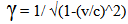 | (24.1) |
The speed of light is predicted to vary over time at the same rate that the speed of an object in motion would change its velocity, resulting in… | (24.2) |
This means that Gamma would always maintain its relative value with the passage of Absolute time. The effects of Special Relativity are locally preserved over time.Also, as the model is developed in successive papers, the relationships of special relativity will have a physical basis with a simple to understand explanation for a variety of situations.
24.2. General Relativity
First it must be noted that nothing in the model proposed so far has run counter to the principals of general relativity, when local or relative measures are used. General Relativity is expressed mathematically in terms of local measures of distance and time. Since local measures of length and time stay proportionally the same, local applications of General Relativity remain unaffected. The spatial relationships between mass and spacetime are still valid locally. Also the same fundamental understanding about the structure of spacetime interacting with the structure of mass is still the same so long as local measures are used to describe local relationships and no long term predictions are made. Secondly, it could be argued that Newtonian or a Keplerian model is actually the more accurate model upon which the Laws of Nature are established. Special relativity and General Relativity could be considered an effect on the basic structure of reality that occurs when the field defining Space is distorted, similar to the way a beam deflects when a load is applied. The basic structure of the beam is simple; defining the shape of the beam in response to stress is a bit more involved. Those who are well studied in General Relativity may have a difficult time considering the validity of this paper. The investment of one’s lifetime to the study of a particular technique that initially seems to correlate to much of Cosmology establishes a strong bias. The expectation for a mathematical model that uses tensor analysis is entrenched. Even the Copernican model used the same mathematical foundation of epicycles and offsets used in the Ptolemaic system. It would not be expected that a new theory would resort to a simpler methodology more akin to the works of Kepler and Newton.There is a reason Gravity has never been incorporated into the other fundamental forces of nature, despite over 100 years of intellectual effort of thousands of very capable people. Change is a difficult task master.
25. Cosmological Measures of Distance and Time
Local measures of distance and time were shown to always remain proportionally the same. But what happens when a local clock or local ruler is used to measure Cosmological objects, i.e. objects observed in the past, deep in space. Are the faster clock rates in the past observable? What about time dilation? How far away in time and distance are the galaxies actually away from us?Cosmological Distances and Cosmological TimeLocal measures of Cosmological Distances and Time are identical to Absolute measures when the reference clock and ruler are established in the present. Referring back to Figure 7 on the light clock, it can be seen that in the present, the length of the light clock and the interval of time defined by the light clock, will always be observed to be constant. Figure 12 is an “Eye of God” perspective where 8 light clocks can be seen in the present without any delay. (Each black bar represents a light clock of some length, say 1 light year, or 10 million light years.).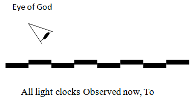 | Figure 12. Light Clock in the present |
Figure 13 is an “Eye of God” perspective of the same chain of consecutive light clocks but this time it is being observed at T1. At all times there is always a string of 8 light clocks strung end to end. 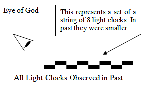 | Figure 13. Light Clocks in the Past |
Figure 14 illustrates what a local observer would see when looking down the chain of 8 light clocks into the past. The light has traveled the length of 8 light clocks with each light clock being smaller the further it is in the past. What the observer is seeing is the distance to the B as it was in the past. Also the local observer is seeing the object 8 light years away in the present.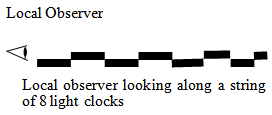 | Figure 14. Look Back Time |
25.1. Variation from the LEM
This is a rather dramatic change from the Limited Expansion Model with commoving coordinates. For example, when the size of the Universe is described in the LEM, the present size would be greater since we are observing the location of the galaxies where they were in the past. The current location of galaxies in the present would be further away since spacetime has expanded during the time it took for the light from distant galaxies to reach us. Wikipedia as of December 6, 2013, places the present size of the Universe as 46.6 billion light years. [8]This “Commoving” or “proper” distance corresponds to the “Eye of God” perspective where the size of the Universe can be seen as it is now, with no time delay waiting to see the distant galaxies across time based on the assumption that the chain of light clocks have remained fixed over time.
25.2. Something “off “ with LEM and Expansion
From a philosophical perspective, the LEM description of the measures of the Universe’s expansion seems off. If a string of light clocks are placed between two galaxies, each mirror would be carried by the expansion of Space, similar to how the galaxies are carried by the expansion of space. The interval of time and distance defined by the light clock, according to the LEM would increase due to the expansion of Space. However, shouldn’t a light clock keep its local measure of an interval of time? Isn’t a light clock a fundamental tool used to define specific intervals of distance an time? Shouldn’t its measure be independent of where the ruler is located?
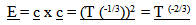
26. Look Back Distance and Look Back Time
The following figure illustrates the relationship with the historical location of a point, to the age of the Universe. Since Distance and time are geometrically connected by the speed of light, a look back distance of 1 light year can be equated to a look back time of 1 year.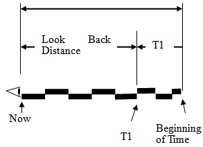 | Figure 15. Look Back Time or Look Back Distance |
 | (26.1) |
27. Problem for GEM, No Expansion!
This perseverance of cosmological relationships presents an issue for the GEM, as presented so far. The following figure shows the location of galaxies within the structure of space. The temporal and spatial separation between each galaxy, (represented by the ovals), is always maintained. This results in no observable expansion! The very foundation upon which the model is proposed becomes non-existent.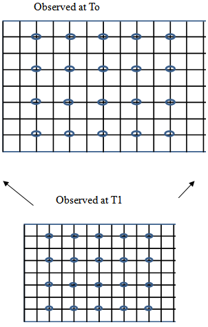 | Figure 16. Galaxies preserve their proportional location over time |
28. More Issues for the GEM - Cosmological Time Dilation
The expansion of space should cause an effect called Cosmological Time Dilation. Physical processes of objects observed in the past appear to transpire slower. One way to visualize time dilation is to imagine an expanding bowling alley, as shown in the following figure. At T1 the two balls are thrown with the same velocity with a 1 second interval between them. As the balls roll down the alley, the alley is stretched. While the balls are rolling down the expanding alley, the distance between the two balls increases. This means that by the time the first ball hits the end of the alley, the second ball must travel further than the distance the two balls started their trip down the alley. The second ball will hit the end of the alley with a greater than 1 second interval of time. This time dilation is proportional to the stretch of the ally, 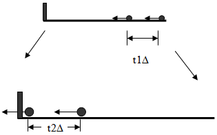 | Figure 17. Expanding Bowling Alley and Time Dilation |
28.1. Cosmological Time Dilation is Observed
Time Dilation is observed at cosmological measures and closely correlates to observation, as per expectations of the current mainstream model. The duration of events are dilated or expanded in close proportion to the cosmological expansion. For example, the light from a “nearby” Type 1a supernova takes about 20+ days to rise and fall. The duration of the light curve increases with the “stretch” of the Universe and correlates to the Cosmological Red shift. If the wavelength of light or spectra of a star is stretched enough to double its wavelength, the duration of the light curve is 2 times longer.
28.2. Except with Quasars
It should be noted that the fluctuations of the energy output from quasars is not dilated in proportion to the cosmological red shift. This observation was made by astronomer. M.R.S Hawkins [6]. Resolving this issue will be a part of the last paper.
28.3. Derivation of Dilated Intervals
The proposed model predicts that since it is light that is transmitting the interval between events observed in the past, the dilation observed will also be effected by the predicted variation in the speed of light. For example, in the bowling ball analogy if the bowling balls also decreased their velocity, it would take longer for the second bowling ball to travel the distance to the end of the ally. The slower speed of light and the stretch of space would cause the Cosmological time dilation.The stretch of space or increase in the distance traveled is… The variation in the speed of light is…
 An interval of time is described by
  | (28.3) |
which leads to the variation in the interval of time as…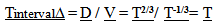 | (28.4) |
For example, an event with a 1 second absolute duration, with the reference for the measure of the interval of time established in the present, is generated when the Universe was 1/8th its present age. What is the duration of the event observed in the present? The distance traveled will be 4 times as long and the speed of light is reduced to 1/2 its present value, so the original event with a duration of 1 absolute second would be observed to now take 8 seconds, 8 times longer.The dilation effect on an interval in the past is the inverse of the Ratio of Time.  | (28.5) |
28.4. The Problem – Dilation is Canceled by Faster Clock Rates
The problem with the GEM, (as developed so far), is that it appears that this dilation is cancelled by the faster clock rates in the past. For example, if the two bowling balls were to be rolled down an alley when the Universe was 1/8th its present age, local clock rates would be 8 times faster in the past. We always us a local clock to establish intervals, not an absolute clock. What locally would appear to be a one second interval of time initially between the two balls, would be 1/8th of a second based on a reference clock established in the present.Time dilation would then expand the initial 1/8th of an absolute second interval of time be measured as 1 second in the present. The two effects cancel, there is no time dilation! This is another problem for the proposed model since time dilation is observed. None the less, what is rather amazing is that the proposed geometric expansion of Space is establishing the structure of the Universe. Order and form are predicted, not only for now, but over time. Even the evidence of the variation in the past is unobserved. The Universe is conforming to a dynamic structure that is almost jewel like. The dimensional relationships of distance and time are corresponding to the structure of the Universe.
29. The Dimensions of Space
The above reference to dimensional relationships needs some clarification since the meaning or meanings of the word “dimension” can be ambiguous. Also, a discussion of dimensions helps provide a more physical understanding of the model.
29.1. Location of a Point
Dimensions are commonly associated with describing the location of a point in space. A traditional dimensional description of a point in a three dimensional space is that from one point to another point that is so far up, or down, left or right, and forwards backwards. (Or, using a polar coordinate system, so far away, with a horizontal and vertical angle measure). Intrinsic to this description is the assumption of a coordinate system, and a method to measure distance and angle measures along the coordinate system.http://en.wikipedia.org/wiki/Dimension_(mathematics_and_physics) [9]
29.2. Physical Properties and Dimensions
Dimensions take on additional meaning when a correlation to a physical property is included. For example, within what is traditionally called a Minkowskian Space, the time interval between points is incorporated in the description of the location a point. This fusion of time in the structure of Space allowed an explanation of the relationships associated with special relativity.http://en.wikipedia.org/wiki/Minkowski_space [10]
29.3. Dimension of Absolute Time and Physical Properties
The addition of an additional dimension of Historical time was established because of the physical correlation of that dimension to the structure of space. The extra dimension was needed to describe physically the way in which relative measures change, despite the fact that locally all relative measures stayed the same. The necessity for the extra dimension can be analogously compared to observing a line along its axis. When viewed from the end of the axis, all points along the axis appear the same, there is no variation. The observation of change along the axis occurs once an additional orthogonal dimension or perspective is incorporated.
29.4. Dimension of Time and Describing a Point’s Location
It has been shown that Absolute time is tied to the physical structure of the Universe but its necessity seems also obvious in the simpler application of dimensions to describe the location of a point. Just as it is important to define the spatial measures, in order to truly define a point’s location, it is also important to define when the measurement is made.
29.5. Physical Criteria for Dimensions
The fact that a point can be expanded to become a line, and a line expanded to become a plane, and a plane expanded to become a 3 dimensional space, and two dimensions of time can be integrated into 3 dimensional space all hint that dimensions are physically associated with the structure of the Universe. Since dimensions are corresponding to the structure of the Universe, it seems prudent to define what a dimension is. The following 4 criteria define a dimension. 1. Dimensions are measures of change. If you can describe how something changes, such as one physical measure compared to another physical measure, then a dimensional relationship is established. How many times I smile in a day would be, by the proposed definition, is a dimensional relationship, the smile dimension. 2. Fundamental or elemental dimensions are the basic or essential relationships used to describe nature. Elemental dimensions are unique, meaning that they are not the result of a combination of two more elemental dimensional relationships. (The smile dimension would not be unique or fundamental).3. Fundamental dimensions are geometric. The relationship of one dimensional measure to another can be described by geometry; you can “draw” the relationship. For example, the speed of light expresses a geometric relationship between distance and time. You can draw a graph illustrating distance traveled over time elapsed. 4. Measures of distance and time reveal the dimensional relationships and the geometry of the Universe. The only “tools” we have to describe the Universe are rulers and clocks. This means that ultimately all physical properties will be a geometric combination of measures of distance and time. The “rulers” used are not just straight, but also measure angular relationships. While the necessity of a separate angular dimension is not obvious in this paper, once quantum properties associated with spin are considered, the equality and necessity of angle and linear rules becomes more evident.
29.6. The Three Physical Dimensions of Spatial Space
The above definition for dimension alters the description of common three-dimensional space. (“small” s). What is understood to be Three-dimensional space is actually described by 3 fundamental dimensions or measures of change between two points. Three different physical descriptions of change are required to describe or locate a point in space. 1. distance, 2. degrees of freedom, and3. sense The dimension of distance (an independent physical property), defines the interval between the two points, the three degrees of freedom (another physical property), yield an orientation in space, and the positive or negative sense determines the perspective within the three degrees of freedom in space. Together these three physical properties allow a point to be located a certain distance away, with the point either located up or down, left or right, or back and forth from an initial point. These three options for physical change correspond to the establishment of a frame of reference. The point being made is that a coordinate system is not the basis upon which nature is constructed. Physical change defines an inherent structure to Space, to which a coordinate system can be attached. The emphasis is not on the reference frame but on the nature of the physical characteristics that allow the use of a reference frame.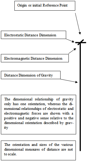 | Figure 18. Three distance Dimensions corresponding to fundamental physical properties, Gravity, charge and magnetism |
29.7. Distance Dimensions for Gravity and Charge
Associating dimensions with physical change is incredibly liberating in that it makes the description of nature much simpler. It also results in increasing the number of dimensions of space. For example, the distance measure for determining gravitational relationships is a different dimensional distance measure used to describe electromagnetic relationships, since each distance measure correlates to a unique physical property. This is illustrated in the following figure.The gravitational distance dimension is larger by about 10^20 times than that of the distance dimensions associated with charge or magnetism. An incremental addition of spacetime on to the additional structure of Space causes a 10^40 times more powerful effect along the dimensional space of charge than it does along the dimensional space associated with gravity.
29.8. More Physical Dimensions - Spin
Spin is a dimensional relationship that is not specifically developed in the model so far, but to not mention it would be a major omission. The “spin” dimension is unique, independent, and geometrically tied to the spatial dimensionsSpin is particularly important the atom. Physical properties of atomic scale objects, such as electrons, protons, and photons, to list a few, have the physical property of spin. Spin is a part of the Fabric of Space. It is generated because of the process of expansion. As a piece of Spacetime is added to the existing structure of Reality, there is a translation or shearing like effect all around the new “piece” when it fits into the existing structure. This shear like effect would correspond to each of the spatial dimensions. This spin dimension would map to each of the three simple spatial dimensions, and with a positive and negative sense.
30. Summary
There following recaps some of the issues and benefits of the model.
30.1. Issues with GEM
There are fundamental issues with GEM, as developed so far. 1. An ambiguous Cosmological Red shift. 2. No observable Cosmological time dilation. The stretch of space which causes time dilation is cancelled out by the faster clock rates in the past. 3. The Universe is no longer measured locally to be expanding. Galaxies keep their location relative to the fabric of space. The relative and Cosmological measures of distance and time between galaxies are always the same when described in the present.
30.2. Benefits of GEM
1. The basic structure upon which the Universe is built is predicted by the proposed Geometric Expansion of Space. Accelerative fields are established as a part of the structure of Space that can be correlated to the fields associated with gravitational effects and the relationships of charge. Gravity is being united with electromagnetism. 2. While little of this paper specifically dealt with the relationships of Quantum Mechanics, it is somewhat obvious that a physical cause can now be attributed to the “fuzziness” or probabilistic characterization of relationships associated at the scale of observation associated generally within the atom. The incremental expansion of Space is being observed. Quantum mechanics potentially has a physical explanation that also integrates with the relationship of Gravity, unifying the two.
30.3. Prediction of GEM
So far the model is proposing a prediction that diverges from the current model. Cumulative measures of Time would be greater than assumed, and should be detectable when physical process that require cosmological periods of time to elapse, such as the evolution of a star.
31. The Snowflake Universe
This expansion or growth of a snowflake is in many ways like the expansion of the Universe. a. The edge of the snowflake (Universe) is where the snowflake (Universe) expands.b. The edge of the snowflake (Universe) is where the present is defined.c. At the edge of the existing structure of the snowflake (Universe) is the location where change can occur. d. The existing structure of the snowflake (Universe) is the accumulation of past events.e. The snowflake (Universe) grows a tiny little piece at a time. The molecule of water (the piece of spacetime) forms on the existing structure of the Snowflake (Universe)f. The “pieces” have a geometric shape that “fit” with the established structure.g. The form or shape of the expansion of the snowflake (Universe) is generally the same across (within) the snowflake (Universe). h. The expansion of the snowflake (Universe) releases energy and it takes energy to change the existing structure.i. The Snowflake (Universe) has Fractal Characteristics. j. The Snowflake (Universe) is Self-similar to a limited extent. The Gravitational distance is similar to the structure of the Charge distance, producing similar dynamically structured relationships at two scales of observation.k. The shape (the dynamics) of the Snowflake (the Universe) conforms to Geometry.
32. Formulas of Observable Space
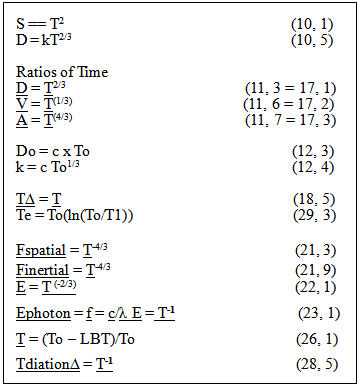
Table 2. Summary of Equations, Expansion of Observable Space
 |
| |
|
33. Expanding the Expansion
The next paper develops the model by expanding the expansion. Just as we can imagine a flatland universe in motion along an unobserved dimension, so too is our observable Universe in motion, (and expanding) along an unobserved dimension. This expansion of the model not only resolves the issues stated previously about the GEM, it also provides a simplification of a number of fundamental relationships of physics.
ACKNOWLEDGEMENTS
I am particular appreciative of the Phil Plait, creator of the Blog “Bad Astronomy”, and Fraser Cain creator of the Space information web site and blog called “Universe Today”. In the past, these sites offered a place for the discussion of alternative models and a source of information. The opportunity to freely discuss my model with others was extremely helpful. Hopefully I will someday get to know some of the members of the blog that took interest in my model people personally, rather than by a user name. It is unfortunate the two sites no longer exist as a place to present or discuss alternative models. At the time of this writing, a highly censored version of the original Blog called, “Against the Mainstream” can be found at a Web Site called “CosmoQuest”. Archived discussions of the model should still be available within CosmoQuest. [10] My user name was Snowflakeuniverse.I must also express my gratitude to Professor Philip D. Mannheim of the University of Connecticut. He granted me the opportunity to present one of the earliest versions of the model to the physics department at the University of Connecticut. Oral presentations are not natural for me and the practice was extremely important. More important, the comments and ideas expressed by those attending were helpful.The template upon which this paper is based was provided courtesy of SAP productions.
References
| [1] | Misner, Thorne and Wheeler, “Gravitation” Pg 719 Figure 27.2 23 printing in 2000). |
| [2] | Bradley W. Carroll and Dale A Ostlie, “An Introduction to Modern Astrophysics”, pg 1116 copyright 1996 |
| [3] | John Hunter of England, Internet presentation of expansion based theory at.. http://www.rescalingsymmetry.com/ |
| [4] | C. Johan Masreliez, Internet presentation of expansion based theory at http://estfound.org/ |
| [5] | Masreliez C.J., The Expanding Spacetime Theory, Astroph. & Space Science, 266, Issue 3, p. 399-447(1999). |
| [6] | M. R. S. Hawkins University of Edinburgh, Royal Observatory, Blackford Hill, EH9 3HJ Edinburgh, UK; mrsh@roe.ac.uk . The Astrophysical Journal, 553:L97-L100, 2001 June 1 © 2001. The American Astronomical Society. All rights reserved. Printed in U.S.A.http://iopscience.iop.org/1538-4357/553/2/L97/fulltext/0151 04.text.html |
| [7] | Age of Universe, courtesy of Wikipediahttp://en.wikipedia.org/wiki/Age_of_the_universe; 7.1. Original source Jump up to: a b c Planck Collaboration (2013). "Planck 2013 results. I. Overview of products and scientific results". arXiv:1303.5062 [astro-ph.CO]. 7.2. Original source Jump up to: a b c Bennett, C.L.; et al. (2013). "Nine-Year Wilkinson Microwave Anisotropy Probe (WMAP) Observations: Final Maps and Results". arXiv:1212.5225 [astro-ph.CO]. |
| [8] | Observable Universe, Courtesy of Wikipediahttp://en.wikipedia.org/wiki/Observable_universe Original source^ Jump up to: a b c Gott III, J. Richard; Mario Jurić, David Schlegel, Fiona Hoyle, Michael Vogeley, Max Tegmark, Neta Bahcall, Jon Brinkmann (2005). "A Map of the Universe". The Astrophysics Journal 624 (2): 463. arXiv:astro-ph/0310571. Bibcode: 2005ApJ...624..463G. doi:10.1086/428890. |
| [9] | Definition of Dimension, Courtesy of Wikipedia http://en.wikipedia.org/wiki/Dimension_(mathematics_and_physics) |
| [10] | Definition of Minkowskian space, courtesy of Wikipedia http://en.wikipedia.org/wiki/Minkowski_space |
| [11] | CosmoQuest http://cosmoquest.org/ Discussions under “Against the Mainstream”, past posting of work have been archived. Search under username “Snowflake Universe”. |
 Abstract
 Reference
 Full-Text PDF
 Full-text HTML