Hicham Hihi
Electrical Engineering Department, LGECOS, Cadi Ayyad University, ENSA, Av Abdelkrim khattabi BP 575 40000 Marrakech, Morocco
Correspondence to: Hicham Hihi, Electrical Engineering Department, LGECOS, Cadi Ayyad University, ENSA, Av Abdelkrim khattabi BP 575 40000 Marrakech, Morocco.
| Email: |  |
Copyright © 2012 Scientific & Academic Publishing. All Rights Reserved.
Abstract
Switching systems are very common in various engineering fields (e.g. hydraulic systems with valves,.., electric systems with diodes, relays,…, mechanical systems with clutches...). Such systems are a particular case of hybrid systems. These systems are characterized by a Finite State Automaton (FSA) and a set of dynamic systems, each one corresponding to a state of the FSA. The change of states can be either controlled or autonomous. The aim of this work is to investigate the structural controllability for controlled switching linear systems modelled by bond graph. Several concepts appeared in the last decade addressing the controllability problem of these systems: controllable sublanguage concept[1], hybrid controllability concept[2], between-block controllability concept[3]. Controlled Switching Linear Systems (CSLS) on which we focus in this work belong to the hybrid controllability concept as they address a reachability problem of hybrid states. In the other hand, the bond graph concept is an alternate representation of physical systems. Some recent works permit to highlight structural properties. In[13], the structural controllability property is studied using simple causal manipulations on the bond graph model. The objective of this work is to extend these properties to CSLS. In this work, the structural controllability of CSLS by means of algebraic and graphical conditions is discussed. First, formal representations of controllability subspaces are given for switched bond graph. They are calculated through causal manipulations. Second, these subspaces are used to propose structured state feedback matrices in the context of pole assignment by static state feedback. Third, a simple example is given to illustrate the previous results. The proposed method, based on a bond graph theoretic approach, assumes only the knowledge of the systems structure. This result can be implemented by classical bond graph theory algorithms.
Keywords:
Switching Systems, Bond Graph, Controllability, Static State Feedback
Cite this paper: Hicham Hihi, Pole Placement of Controlled Switching Linear Systems - Bond Graph Approach -, International Journal of Theoretical and Mathematical Physics, Vol. 3 No. 2, 2013, pp. 81-89. doi: 10.5923/j.ijtmp.20130302.05.
1. Introduction
A broad class of hybrid systems is composed of physical processes with switching devices. Such processes are called switching systems and are very common in various engineering fields (e.g. hydraulic systems with valves,.., electric systems with diodes, relays,…, mechanical systems with clutches...). These systems are characterized by a Finite State Automaton (FSA) and a set of dynamic systems, each one corresponding to a state of the FSA. The change of states can be either controlled or autonomous. Various researchers investigated this problem using the bond graph tool [1,2,3,4,5,6]. The ideal and the non-ideal approaches are used :- In the non-ideal approach, switches are modelled as resistive elements associated with modulated transformer. The modulation is done using a boolean variable. - In the ideal approach, switches commutateinstantaneously. Each switch is modelled as a null source: effort source for a closed switch state, and flow source for an open one. This approach is used in this work.Lately, there have been a lot of studies on stability analysis and design[4]-[5]-[6]. (Liberzon and Morse,[5]) summarize three basic problems regarding stability and design of switched systems. They are: (i) stability for arbitrary switching sequences; (ii) stability for certain useful classes of switching sequences; (iii) construction of stabilizing switching sequences. For problem (i), finding conditions under which there exists a common Lyapunov Function forthe system is a typical approach[6]. For problem (ii), multiple Lyapunov functions method, an extension of classical Lyapunov theory, is the main tool[7]. For problem (iii), there are many results available[4].Petterson and Lennartson in[8] show that the search for Lyapunov functions can be formulated as a linear matrix inequality (LMI) problem. Xu and Antsaklis in[9] give a necessary and sufficient condition for the asymptotic stabilizability of switched systems consisting of several second-order subsystems with unstable foci. If the condition holds, an asymptotically stabilizing switching law can be obtained. Hu, Xu, Antsaklis and Michel in[4] discuss the robustness of this kind of stabilizing control laws.This paper is briefly outlined as follows: The second section formulates the problem. In section three the CSLS algebraic controllability is reviewed. In section four, an asymptotically stable state feedback design algorithm is derived for such systems. In section five, the structural controllability of these systems is discussed, for which, we calculate a formal representation of controllability subspaces of switched bond graph. It allows to propose in section six, the structure of feedback matrices for the pole assignment control problem, this for all modes. Graphical procedures are proposed. Section seven contains an illustrating example. Finally, the conclusion is provided in section 8.
2. Problem Formulation
Consider a CSLS[10], described by | (1) |
Where  is the state variable,
  is the input variable,
  is a piecewise constant switching function and
  the hybrid state. According to values of
  , there exists
  configurations,
  . So
. So and
and  .If we consider this system in a particular mode i, the equation (1) can be written as
 | (2) |
With  and
and  .Remark 1 System (2) can be considered as a linear time invariant system (LTI).Assumptions 11) We suppose that
  and
and  matrices are constant on a time interval
  , where
  , and the constant
  is an arbitrarily small and independent of mode
  . For instance, suppose that the dynamics in (1) are given by (2) over the finite time interval
  . At time
  the dynamic in interval
  is given by
  . 2) We assume that the state vector
  does not jump discontinuously at
  .If we further assume that
  then the following convenient representation of (2) is obtained
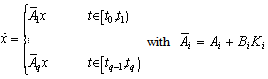 | (3) |
We refer to systems (1) and (3) interchangeably as the switching systems
3. Controllability of CSLS
The controllability of (1) was defined:Definition 1[10] Given any pair of hybrid states, denoted as  and
and  , respectively, if there exists a timed mode-switching set
  and a corresponding piecewise continuous-finite input signal
  , such that system (1) evolving under these two distinct inputs is reachable from
  to
to  within a finite time interval, then the considered system (1) is controllable, otherwise, system (1) is uncontrollable.
3.1. An Algebraic Sufficient Condition
When system (1) has only one mode, the controllability can be analyzed through the controllability matrix (4).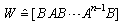 | (4) |
For the general case, a controllability combined matrix  of system (1) is given by equation (5):
 | (5) |
Theorem 1[10] The CSLS (1) with  modes is controllable, if the controllability matrix
  is of full row rank.Remark 2 From this theorem, we can deduce that:1) The system (1) can be controllable, if there is only one controllable sub-system (mode). 2) However, it is possible that no sub-system is controllable but that the system (1) is controllable.
4. Piecewise Constant Controller Design
The controller design is based on placement of all poles of all modes to appropriate positions in the left hand side of the s-plane. In[11] the following lemma is proposed: Lemma 1[11] Given a controllable LTI system (A, B) in controller canonical form, i.e., 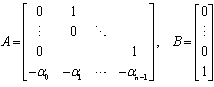 and a scalar h > 0, for any
  , there exists a constant state feedback
  such that
 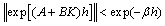 | (6) |
This lemma can be extended to a more general case, which is the starting point to design the piecewise constant state feedback controller.Lemma 2[12] Given a controllable LTI system  and a scalar h > 0, for any
  , there exists a constant state feedback
  such that
 | (7) |
4.1. Asymptotic Stability
Based on Lemma 2 and if each subsystem  is controllable, Xie and al in[12] gave the following theorem:Theorem 2 For the system (1), and for each subsystem
  there exists a state feedback
  such that the closed loop system
 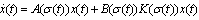 is asymptotically stable. Since each subsystem
  is controllable, suppose:
  . Denote
 Then
Then  is nonsingular. Using lemma 2 and theorem 2, an asymptotically stable state feedback controller design procedure can be constructed[12].Procedure 1 For the system (1), for each subsystem
  , a state feedback matrix
  such that the closed-loop system is asymptotically stable can be calculated as follows.1) Determine the nonsingular matrix
  such that
  is in controller canonical form, where
  ;2) Calculate
  ;3) Select
  such that
  , moreover, let
  for
for  ;4) According to
  , calculate the state feedback matrix
  ;5) Let
  .In the next step structural controllability of CSLS modelled by bond graph is studied.
5. Bond Graph Approach
The structure junction of a switching bond graph can be represented by figure 1[14]. Five fields model the components behaviour, 4 that belong to the standard bond graph formalism: - source field which produces energy, - detector field; - R field which dissipates it, - I and C field which can store it, and the Sw field that is added for switching components. This element (Sw) is made of the power variables imposed by the switches in the chosen configuration.Figure 1 represents the block diagram that is deduced from the causal bond graph.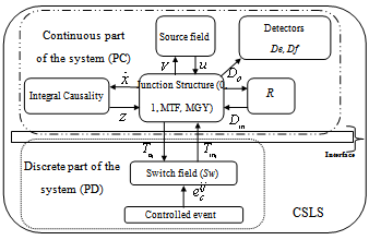 | Figure 1. Structure junction |
The following key variables are used :- the state vector x(t) is composed of the energy variables on the bond connected to an element in integral causality (the momenta  on I elements and charges
  on C elements), and the complementary state vector z(t) is composed of power variables (the efforts e on C elements and flows f on I elements); -
  and
and  represent the variables going out of and into the R field; - the vector u(t) is composed of the sources; -
  is composed of the zero valued variables imposed by the switches in this configuration; -
  is composed of the complementary variables in the switches; - the vector y(t) is composed of the continuous outputs.Assumptions 2To take into account the absence of discontinuities (Assumption 1), we suppose that there are no elements in derivative causality in the bond graph model in integral causality, before and after commutation.Using this structure, the following equation is given[14] :
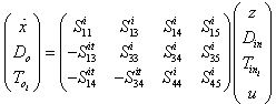 | (8) |
Let the constitutive law of the  field be linear:
  .
.  is a positive matrix, with
  . Let assume that
 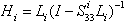 is an invertible positive matrix.In a linear case, the law constitutive for the fields of storage
  and
and  can be written :
  . Where F is a symmetric positive definite matrix.Then the second row leads to
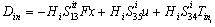 The third line of (8) gives:
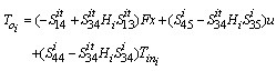 | (9) |
The substitution in the first line of (8) gives: 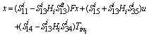 | (10) |
Then, we have:  | (11) |
This system is equivalent to system (2), where  ,
,  and
and  .When the elements of commutations are in the chosen configuration (mode i for example), then
  .Therefore, for
  switchs, we have
  modes:
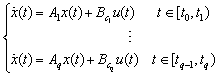 | (12) |
This system is equivalent to system (1).
5.1. Structural Controllability
The bond graph concept is an alternate representation of physical systems. Many works allow to highlight structural properties of these systems[13]-[14]. In[13], the structural controllability property is studied using simple causal manipulations on the bond graph model. This result was extended to case of CSLS[14]. Our objective is to use the latter result for to propose structured state feedback matrices in the context of pole assignment by static state feedback.In the following we note that:-BG: acausal (without causality) bond graph model,-BGI: bond graph model when the preferential integral causality is affected,-BGD: bond graph model when the preferential derivative causality is affected,- : the number of dynamical elements remaining in integral causality in the BGD of mode i. -
  : the number of dynamical elements remaining in integral causality in the BGD after the dualization of the maximum number of input sources in order to eliminate these integral causalities.
5.1.1. Graphical Sufficient Condition 1
A system (1) with q modes is controllable if only one system is controllable. This condition can be interpreted by using the result of structural controllability of LTI system.Indeed, this result is a simple recovery of those giving the necessary and sufficient condition of structural controllability of LTI system modelled by bond graph approach.Theorem 3[14] The CSLS system (12) is structurally state controllable if:1- All dynamical elements in integral causality are causally connected with an input source.2- BG-rank .Property 1[14] BG-rank
 .To study the controllability of system (12), it is necessary to apply this result to all modes; if one controllable mode exists, the procedure is stopped.The case where no mode is controllable, but when the system is controllable, can be verified by formal calculation of combined matrix (4). This calculation can be formally effected by using the bond graph model in integral causality or by calculating the controllability subspace from bond graph model in derivative causality. We chose to translate the latter in the form of a second sufficient condition.
5.1.2. Graphical Sufficient Condition 2
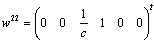
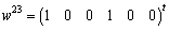
Thereafter, formal representations of controllability subspaces, denoted as  , are given for bond graph models. They are calculated through causal manipulations. The bases of these subspaces are used to propose a procedure to study the controllability of system.On the BGDi (and dualization of input sources) there exists
  elements remaining in integral causality and
  elements in derivative causality.
 algebraic equations can be written (equation 13):
 | (13) |
-  is either an effort variable
  for
for  -element in integral causality or a flow variable
  for
for  -element in integral causality;-
  is either an effort variable
  for
for  -element in derivative causality or a flow variable
  for
for  - element in derivative causality;-
  is the gain of the causal path between the
 or
or  -elements in integral causality and the
 or
or  -elements in derivative causality.Let us consider the
  row vectors
  whose components are the coefficients of the variables
  in the equation (13).Property 2 The
  row vectors
  are orthogonal to the structural controllability subspace vectors of the
  mode. We write
  and
and  .Using the bond graph model in derivative causality, the uncontrollable
  subspace can be calculated[14]. Procedure 2 Calculation of
  1) On the BGDi, dualize the maximum number of input sources in order to eliminate the elements remaining in integral causality,2) For each element remaining in integral causality, write the algebraic relations with elements in derivative causality (equation 13),3) Write a row vector
  for each algebraic relation with the causal path gains and write
  .In order to calculate an
  basis, it is enough to find
  independent column vectors
  . These vectors are gathered in the matrix
  .From the BGDi (and dualization of inputs sources),
  algebraic relations can be written (14).
 | (14) |
- is either a flow variable
  for
for  -element in derivative causality or an effort variable
  for
for  - element in derivative causality;-
 is either a flow variable
  for
for  -element in integral causality or an effort variable
  for
for  - element in integral causality;-
 is the gain of the causal path between the
  element in derivative causality and the
  element in integral causality. Suppose now
  column vectors
  whose components are the coefficients of
  and
and  variables in equation (14).Procedure 3 Calculation of
  1) On the BGDi, dualize the maximum number of continuous input sources in order to eliminate the elements in integral causality;2) For each element in derivative causality, write the algebraic relations with elements in integral causality (equation 14);3) Write a column vector
  for each algebraic relation with the causal path gains (equation 14), with
  .Property 3[14]
  column vectors
  compose a basis for the structural controllability subspace of
  mode.The graphical calculation of structural controllability subspaces and theorem 1 leads to theorem 4:Theorem 4[14] If rank
 , the system CSLS (12) is structurally controllable.
6. Pole Assignment
Now, we suppose a monovariable (m=1) linear sub-system (mode i), that is ( ) in equation (1). The problem is to find a state feedback law
  to each mode i in the time interval t[ti-1, ti) such that the closed loop state matrix
  has the desired poles. In fact, the number of assignable poles is equal to the rank of the controllability matrix, this for each possible mode. It is deduced that the number of independent parameters in the matrix
  is equal to the controllable subspace in mode i. The objective is to find these parameters.We recall some relations
  {Wi} and
  . We can write:
 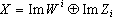 with X the state space, and
  .Now, we calculate
  . The roots of this characteristic polynomial are the closed loop roots.First, the different matrices are decomposed. A permutation between the dynamical elements enables us to write
  with
with  such that in the state vector, the
  first variables are the non-controllable variables, which are the dynamical elements which remain in integral causality in BGDi model. The following variables are the dynamical elements appearing in the algebraic relations after BGDi and dualization.Suppose now this new matrix :
 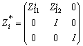 With
With  and
and  is identity matrix. The matrices
  and
and  are decomposed as
  .
. 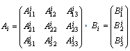 and
and 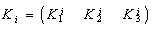 Then, the characteristic polynomial of
  is :
is :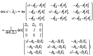 From the relation
  , we obtain :
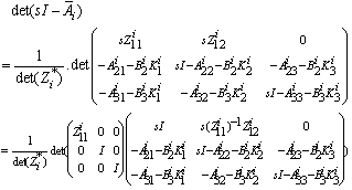 After manipulations, we have
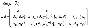 With
With  Then
Then  becomes
  . The pole assignment problem consists in calculating
  and
and  , with
  . It comes
  . The
. The  non-controllable poles are equal to zero, because they correspond to zero eigenvalues of the state matrix.Proposition 4 For each mode, the independent parameters of the closed loop characteristic polynomial
  are the parameters of the two matrices
  and
and  .Now we write
  and we calculate
  directly from the controllability space matrix
  . It is possible to write
  as :
as :  From the relation
  . Then we have
 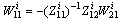 and
and 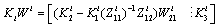 ,
,  is a square matrix and can be chosen invertible, and equal to the unity matrix, because
  has maximal rank. In fact, it is enough to keep only the minimum number of independent parameters in the matrix
 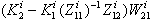 .
.
7. Example
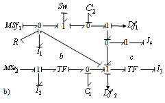
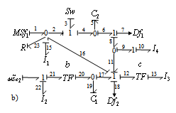
Let us consider the following acausal BG model :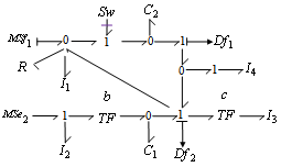 | Figure 2. The acausal Bond Graph |
This model contains one switch, then we have 2 possible configurations (mode F:  :
:  , mode E:
  :
:  ). ■ The BGIi of these modes are shown in figure 3.
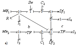 | Figure 3. a) BGI of mode F |
 | Figure 3. b) BGI of mode E |
There are six state variables  on
on ,
,  on
on 
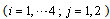 . The dimension of the system is
  . For models
  and
and  all state variables are causally connected with the sources, and are in integral causality. There is no storing element in derivative causality in these configurations, so the state variables are given by :
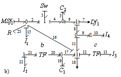
 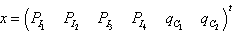 .■ The BGDi and dualization (figure 4).
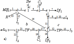 | Figure 4. a) BGD of mode F |
 | Figure 4. b) BGD of mode E |
• For mode FThe element  is in integral causality, we can write
  , thus
  .The four dynamical elements
  and
and  are not causally connected with
  , we can write
  . The four corresponding vectors are
 ,
, ,
,  and
and  . The algebraic equation corresponding to the element
  is given by:
  . Then
  and
and  .We have
 , this mode is not controllable.• For mode EAfter commutation, we pass in mode E and we have
 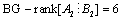 . The mode E is controllable by two inputs, then this system is controllable.Case : m=1 (Monovariable system)In this part, we eliminate the second source and we affect the derivative causality (and dualization) on the BG model.■ The corresponding BG models are drawn on figure 5.
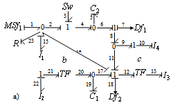 | Figure 5. a) BGD of mode F |
 | Figure 5. b) BGD of mode E |
We have 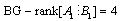 and
and  , these modes are not controllable.• For mode FThe elements
  and
and  are in integral causality, we have
  and
and .The two dynamical elements
  and
and  are not causally connected with
  and
and  , we can write
  , the two corresponding vectors are
  and
and  . The algebraic equations corresponding to the elements
  and
and  are given by:
 and
and  and
and .• For mode EThe element
  is in integral causality, thus we have
 and
and  . The two corresponding vectors are
  and
and  . The algebraic equations corresponding to the elements
  and
and  are given by:
  ,
,  and
and  ; then
 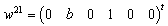 ,
,  ,
, and
and 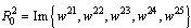 .We apply theorem 4, we have
  , this system is controllable.The studied system has two modes, Suppose
  and
and  .For mode F there are two uncontrollable states variables associated the dynamical elements
  and
and  , and for mode E there is one uncontrollable state variable associated the dynamical element
  . We conclude that for mode F,
  and
and  can be arbitrarily chosen, from the same manner for the variable
  in mode E. The four (respectively five) independent coefficients of the state feedback matrix are highlighted
  and
and  . These coefficients are the unknown parameters for the pole assignment problem relating to each mode. They are the parameters of the characteristic polynomial of the state matrices
  .Case : m>1 (Multivariable system)The minimum number of parameters in the state feedback matrices for the pole assignment problem is n. In case of multivariable systems, the choice is not unique even for controllable systems. Suppose now the BG model (mode F and E) (figure 3). Suppose
 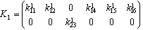 and
and 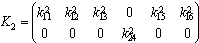 . For mode F there is one uncontrollable variable associated the dynamical element
  and for the mode E all the variables are controllable. We conclude that for mode F,
  can be arbitrarily chosen,The state feedback matrices can then be
 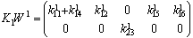 and
and 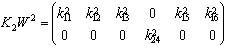 .
.
8. Conclusions
This paper has studied the controllability property of a class of switched linear systems with the aid of simple causal manipulations on the bond graph model. Thus, formal calculation enables us to know the reachable variables, its checking is immediate on the BGI; on the other hand the BGD enables us to characterize from a graphic point of view the whole of the subspaces that are controllable with respect to each mode. While employing these subspaces, we have proposed a simplified state feedback matrices for the pole assignment problem, this for all the possible configurations of the system. The application was made on an example. The problem is now to highlight more structural information in order to solve other current questions from a structural point of view. It will be done in a future work.
References
| [1] | J. A, Stiver, and P.J, Antsaklis, "On the controllability of hybrid control systems,” In Anon (Ed.), Proceedings of the 32nd conference on decision and control, San Antonio, Texas (pp. 294-299), (1993). |
| [2] | M, Tittus, and B. Egardt, "Control design for integrator hybrid systems,” I3E Transactions on AC, 43(4), 491-500, 1998. |
| [3] | P.E. Caines, and Y.J. Wei, "Hierarchical hybrid control systems,” a lattice theoretic formulation. I3E Transactions on AC, 43(4), 501-508, 1998. |
| [4] | B. Hu. X. Xu. P. J. Antsaklis. and A. N. Michel, “Robust stabilizing control laws for a class of second-order switched systems”. Sys and Contr Letters, 1999, v38, n2. pp. 197-207. |
| [5] | D. Liberson and A. S. Morse. (1999) “Basic problems in stability and design of switchcd systems”. IEEE Contr. Syst. Mag. vol.19, no.5.pp.59-70. |
| [6] | D. Liberson, D. J. P. Hespanha. and A. S. Morse (1999) “Basic problems in stability and design of. “Stability of switched systems: a Lie-algebraic condition”. Systems Contr Lett, vol, 37,no. 3, pp. 117-122. |
| [7] | H. Ye, A. N. Michel and L. Hou “Stability theory for hybrid dynamical systems”, IEEE Trans. Automat. Contr. 1998. vol.43, no 4, pp.461-474. |
| [8] | S. Petterson. and B. Lennartson.”Stability and robustness for hybrid systems”. Proceeding of the 35th IEEE Conference on Decision and Control, Kobe, Japan, 1996, pp. 3202-1207. |
| [9] | X. Xu and P. J. Antsaklis. “Design of stabiling control laws for second-order switched systems”. Proceedings of the 14th IFAC, Beijing, China.1999. vol. C, pp, 181-186. |
| [10] | Z. Yang. An algebraic approach towards the controllability of controlled switching linear hybrid systems. Automatica, 38 :1221-1228, 2002. |
| [11] | Q. Zhao and D. Zheng “Stable and Real-Time Scheduling of a Class of Hybrid Dynamic Systems”, J. DEDS, 1999, vol. 9, no. 1. p.45-64. |
| [12] | G. Xie and L. Wang “Controllability Implies Stabilizability for Switched Linear Systems Under Arbitrary Switching”, ISIC, Houston, Texas, Octobre 2003. |
| [13] | C. Sueur and G. D. Tanguy. Bond Graph approach for structural analysis of MIMO linear systems. J.Franklin.Inst, Vol.328, 1, 55-70. 1991. |
| [14] | H. Hihi, “Switched Bond Graph Determination of Controllability Subspaces for Pole Assignment“, I3E, SMC, Alaska, October, 2011. |
 Abstract
 Reference
 Full-Text PDF
 Full-text HTML