1. Introduction

Mathematics has lots of implicit and explicit assumptions. The major idea that we want to establish is that nature does not and cannot make any assumptions; therefore mathematics cannot be used to describe nature. Contrary to the common understanding that these assumptions are for approximations; in reality their removal can dramatically change the outcomes. One example is the infinity assumption in FT. You make it finite then there will be no uncertainty, as we show. During the last 50 years engineering technology has significantly advanced due to the advent of microprocessors. On the other hand our mathematics, did not keep pace with it, and is still using 100 and even 200 years old concepts. The ideas and philosophies of simpler requirements of those days are deeply embedded in this mathematics. A 100 year old theory cannot be used in modern technology. We show that the idea – whatever happens in mathematics will happen in nature – does not have any experimental foundation.

We describe some laws of nature that are quite obvious but we have never formally included them in our physics and mathematics textbooks. However, these lawsareimplemented in all embedded engineering systems, which are built around microprocessors, electronic digital and analog hardware, embedded software, and multitasking real time operating systems (RTOS). These laws are necessary in thistechnology to satisfy modern complex engineering requirements. These embedded systems are part of nature, because they are built using objects of nature, and they also interact with nature using analog to digital and digital to analog converters. In this paper, we use these embedded systems as representatives of nature, to explain nature, and to test our theories. We show that they are immensely complex, and yet are of significantly lower level of sophistication compared to real nature.

It is well known that these embedded systems are full of patches and kludges, and therefore are very unreliable, unpredictable, and crashes quite often. These engineering products are made to work by using multiple redundancies, including automatic hardware-software resets by watch dog timers. More details of this specific engineering problem have been presented in Das¹. All these failures happen because it uses math and science theories that were developed 100 years before. Yet these embedded systems do not contradict nature, but truly represent nature, do not make any assumptions, and can be used for testing our theories. Once we understand these laws of nature, we will realize that mathematics cannot be used to describe nature. Use of mathematics to describe nature is itself an assumption. Although our focus in this paper is uncertainty principle, but since we are searching for the root cause of this uncertainty, and its testability, we have to feel the complexity of nature and then realize the limitations of mathematics. We illustrate this concept of unsuitability of mathematics, by often using the embedded engineering systems, which are manmade copies of nature.

Thus we observe, very similarly, that no physical experiment, which is also an engineering experiment, can verify any scientific theory. The reason is quite simple and obvious. Since engineering products obey all laws of nature, therefore they cannot make any assumptions, because nature does not and cannot make any assumptions. On the other hand all theories of mathematics and science have assumptions. Thus all experiments inherently and automatically eliminate all assumptions from a theory, so the theory becomes invalid. Without assumptions these theories are not meaningful. Therefore experiments are not really testing any theory.

To avoid any confusions and misinterpretations, we examine many published proofs of uncertainty principle, (including the one given by Heisenberg), from many different references to convince the reader that the uncertainty principle has nothing to do with physics or nature but is a property of Fourier Transform and other mathematics. We show its equivalence with concepts like time-bandwidth product or dimensionality theorem as used in digital signal processing and communication engineering. They are all based on the same infinite time property of FT, as described in Das². All these results change when we replace the infinity by finite values in the definition of FT. The new results become more meaningful and useful also. Besides FT, there are other proofs of uncertainty principle, like operator theoretic. We investigate them also in this paper, and highlight the assumptions behind them, contrasting with these laws of nature.

The paper is organized in the following way. We start with some definitions, for differentiating and comparing: math, science, engineering, and nature; and also for testing concepts. Then we briefly describe some laws of nature that embedded engineering is forced to implement, to make engineering work with nature. The first proof of uncertainty principle that we provide is taken from Heisenberg’s book. Then we take another proof from a newer textbook on quantum mechanics. These two proofs and their similarities will convince the reader that the uncertainty principle is based on FT theory and has nothing to do with nature. We also examine the proof based on operator theory and the hidden assumptions behind it. Uncertainty principle is also widely used in engineering and we explore their proofs and show that they are all based on FT. Finally we show that by eliminating infinity assumption from FT we can remove the uncertainty.

2. Definitions

We want to convince the reader that engineering really knows the nature better than any branch of human research activities. This is so because, all engineering activities make products out of objects taken from nature. Therefore a product cannot be made that violates any laws of nature. Thus engineering cannot make any assumptions about nature. We give some basic definitions to clear the perspective.

Nature has only two kinds of things; some objects (living and non-living) and some actions. Actions are like forces of nature and have some energy associated with them. In some sense actions are characteristics of objects also. For example light energy is a characteristic of sun; similarly wind force is a characteristic of earth.

2.1. Definition of Laws of Nature

The laws of nature are the universal characteristics of the objects of nature. They exist independent of human experiences and assumptions.

Everything that we see around us is engineering. The cars, airplanes, roads, buildings are all products of engineering. A product is a physical hardware that we can see and touch.

2.2. Definition of Engineering

It is a process that is required to create an useful product.

Thus engineering is not the textbooks on engineering subjects, like mechanical, electrical, etc. All products use objects of nature, and therefore all products also obey laws of nature. Thus we can define science in the following way.

2.3. Definition of Science

It is a collection of manmade theories that tries to explain the laws of nature.

2.4. Definition of Mathematics

It is a symbolic language, used to describe expressions of natural language. Its main purpose is to justify the scientific theories.

Consider an example to clarify the distinction between science and engineering. If we place a magnetic needle under a wire, and pass current through the wire, then the magnet will be deflected. We call this an engineering experiment. It is a product that we can see, touch, and learn about it; and it does something useful also. The process used to demonstrate this needle movement is engineering. The science part says that the magnet has a field called magnetic field, the electricity creates a field called electric field (or may be a magnetic field); these two fields interact and create a force that deflects the magnet. Thus when Newton is making a lens he is doing engineering, when he is proposing corpuscular theory of light he is a scientist, and when he is writing f=ma he is a mathematician.

2.5. Definition of Theory

A Theory is (a) a collection of assumptions and (b) a collection of conclusions that only hold under the assumptions.

It appears that all theories have assumptions. Somehow mankind forgot to realize that assumptions are not acceptable to nature, until we encountered modern software based engineering technology, which failed to incorporate such theories. The truth is: nature does not and cannot make any assumptions.

2.6. Example of a Theory

Newton’s First law: (a) In the absence of any interaction with something else (b) An object at rest will remain at rest (c) An object in motion will continue in motion at constant velocity, that is, in constant speed in a straight line

The item (a) in the above law is the assumption. The items (b) and (c) are the conclusions. The last two items will be valid only when the first item (a) is valid. A theory has two parts, if any one of the two parts fails then that theory will be invalid and we will say that the theory does not work in engineering or simply does not work.

2.7. Definition of Invalidity

A Theory is invalid if (a) Its assumptions cannot be tested or implemented or (b) Its conclusions cannot be verified by any experiment

Incidentally, we all know that Newton’s first law cannot work in nature, because of the assumption it makes. Here is a physics textbook by Ferraro³, which says on page 8 - “We could hardly sustain that this principle [First law] is a strict experimental result. On the one hand it is not evident how to recognize whether a body is free of forces or not. Even if a unique body in the universe were thought, it is undoubted that its movement could not be rectilinear and uniform in every reference system”. Many such examples on assumptions can be found in Das¹.

2.8. Testing a Theory

In many cases we see that experimental results seem to suggest that the theory is correct. But that is not a verification of a theory. All experiments are engineering experiments. Engineering is part of nature and therefore obeys the laws of nature. Since nature does not and cannot make any assumption, all experiments automatically eliminate all assumptions of all theories. Therefore experiments do not and cannot prove theories.

To test a theory, which claims to be a law of nature, we must first establish the environment, to verify the assumptions in nature, and not in an artificial environment. Then we must test the results or conclusions under those assumptions. As an example, Newton's First law can never be tested, because it has an assumption - "In the absence of any interaction with something else". This assumption is never valid in nature. Gravitational force is always there in space and near earth. So, according to our definition of invalidity, this First law is false. Note that this law is not an approximate theory either. An object left stationary in space will not remain stationary, and will soon start moving and reach very high speed on a curved trajectory. We give another test example later for the operator theoretic approach.

Same is true for uncertainty principle which, as we show, uses Fourier Transform (FT). The FT uses infinite time assumption. Since we can never perform an experiment for infinite time, we can never verify uncertainty principle. If we replace infinite time by finite time, we will not get an approximate result, as we show there will be no uncertainty, a dramatic change. Thus in reality, we have never tested the uncertainty principle.

All we want is to make the readers understand, that assumptions are invalid in engineering, and therefore in nature also; and thus assumptions cannot be used to describe a law of nature. We claim that all mathematics and therefore sciences have assumptions. Therefore no theory can be tested using any experiment, because all experiments will eliminate all assumptions, thus making the theories not testable and therefore invalid.

3. The Laws of Nature

In this section our objective is to show that mathematics cannot be used to describe nature. Therefore what happens in mathematics will not and cannot happen in nature. We have three main points to convince the reader about this objective. (A) Mathematics uses lots of assumptions, but nature does not. Thus inherently mathematics violates the laws of nature. (B) Mathematics is a symbolic language, and is not capable of presenting our ideas, thoughts, and intelligence. We cannot even express our feelings successfully using our oral language, then how can we express ourselves using a symbolic language like mathematics. (C) Nature is immensely complex. We do not have even enough intelligence to understand it. Nature has created humans, it is therefore impossible for us to comprehend nature. It is similar to the case that our computers will never be able to understand us. Thus what we do not understand, the nature in this case, cannot be described by mathematics.

In this section we present the following new laws of nature: (a) boundedness law (b) finite time law (c) simultaneity law and (d) the complexity law. We describe them in some details in the subsections below. More can be found in Das¹. We discuss these laws mostly using engineering examples and context. A little imagination will reveal that they are more complex in real nature. We will make more comments later – about the use of mathematics for nature - which will require an understanding of the complexity of nature. If manmade engineering, which is part of nature, can be so complex then you can imagine how complex the real nature can be.

This section addresses three important issues. (A) We show that these are laws of nature, and they are implemented in all modern engineering systems. (B) Mathematics violates all of these laws. Therefore mathematics cannot describe nature. (C) All engineering experiments to test mathematics and science will fail. These laws will not allow the assumptions in engineering. Since these are laws of nature, the nature will similarly remove all assumptions, and thus invalidate the theories, since the theories work only under their assumptions.

3.1. Boundedness Law

This law shows that every engineering system is non-linear by design. It will be clear that nature also obeys this law. Most of the mathematical theories that we use in quantum mechanics (QM) like Fourier Transform, Laplace Transform, Linear ordinary and partial differential equations like Schrodinger’s equation, linear operator theory, Hilbert space, inner products, all violate this law of nature and therefore cannot be used to describe nature. Their use in uncertainty principle to characterize nature cannot be correct. These theories require linearity assumptions. Moreover this law prevents infinity assumptions also. In this sense linearity automatically assumes infinity.

Let x denote any physical variable, like voltage, current, water pressure, position, velocity etc. In engineering and in nature also, x always has a lowest and a highest possible value. Or in other words they cannot take any arbitrary value from -∞ to +∞. We call this feature of a variable as the boundedness law of nature. In engineering they are also known as nonlinearity or saturation or limiter law. Using mathematical notations we can express this law in the following way:

(1)

Here L can be positive, zero, or any negative number but cannot be minus infinity. Similarly U can be negative, zero, or any positive number, but cannot be positive infinity. However U must be greater than L.

Figure 1 describes graphically the logic to implement (1). The horizontal axis is the input axis for the variable x. Along the horizontal axis, x can take any value from minus infinity to plus infinity. We show the boundedness of x in the vertical or output axis of the graph. The graph shows that when x is between a and b, whatever way x changes, similar changes happen in the output axis. However, when x goes beyond b you can see that on the output axis it stays fixed at U. That is the output is limited to U. The same is true in the lower direction of x, and is limited by L. The box in Figure 1 represents a non-linear system.

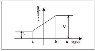Figure 1. Saturation Non-Linearity

Wherever there is an engineering variable in a system, an embedded engineer adds this box at that location of the system, to protect the components there, otherwise the system will fail or burnout. This box is implemented in analog hardware circuits in the form of automatic gain control. It is also implemented in both digital hardware and embedded microprocessor based software. All hands-on experienced engineers will automatically place these boxes in their design. This is a very common embeddedengineering practice. We should know that local linearization cannot work in engineering, see Das¹ for details.

Since the box is a nonlinear box representing the natural law, and implemented by design, all engineering systems are nonlinear systems. Or in other words there are no linear systems in engineering and in nature. It is clear that this is a law of nature. No variable or object in nature can violate this boundedness law. However mathematics and science have largely ignored the boundedness law. Thus this law will prevent testing of any mathematical theory.

3.2. Finite Time Law

Finite time is a law of nature. In fact we should recognize that infinity is invalid for mass and length dimensions also, just for the same reason for time dimension. Time here is defined and measured as the period between two events. In this sense, this law includes the boundedness law also. The FT, Operator theory, Hilbert space, inner products, Schwartz inequality, use infinity in their definitions. Thus their applications cannot be valid for nature. Also they cannot be tested, because all engineering products use finite values. Any time we try testing a theory, the test will eliminate all assumptions of the theory, including infinity. Since we cannot perform a test for infinite time, we really have never tested the uncertainty principle.

Although the earth is going round the sun forever, but we see the rotation around sun, and the rotation around earth’s own axis, are finite duration activities. Everything in nature goes through a birth process, maturity process, and death process. All these processes are finite duration activities. Our physicists have detected the birth and death of stars. Human lives are no exception to this finite duration activities. We should recognize that a distance of a billion light years is also a finite number. The mass of a galaxy is also finite. The time between birth and death of a star is finite. Although our systems run continuously, like GPS transmitters and receivers, traffic light systems at street corners, but if you look at the internals you will always find that the building blocks are based on finite duration processes.

These days most of the complex engineering systems are controlled by one or more digital microprocessors and software. All activities that these systems perform are done in small interval of time duration, of the order of several micro or milliseconds. And such activities are repeated continuously as detailed in Das¹.

Consider the example of a robotic arm, picking up an item from one place and dropping it in another place and repeating the process in, say, less than a second of time. Similarly, a digital communication receiver system, like GPS, receives an electrical signal of microsecond duration, for example, representing the data, extracts the data from the signal, sends it to the output, and then goes back to repeat the process.

Our embedded software runs under real time multitasking operating systems which are also nothing but finite state machines. A finite state machine is a collection of finite number of activities of finite durations, repeated asynchronously and/or synchronously based on the external as well as internal events. Every time a task returns, it finds a different environment. The previous tasks have operated on the system and created a new environment. Thus the same finite duration task or activity is always performed on different signal and under different environment. Thus system is changing after every finite interval. The same is true for nature.

Note that for any practical applications a large number can be considered as infinity. When we replace infinity by this large number, however, the characteristics of the original mathematical theory dramatically change, as we show in this paper using the case of Fourier Transform (FT). In case of FT, we show that uncertainty goes away. In case of Laplace Transform, see Das¹ for example, the complex plane becomes analytic, when we eliminate infinity. Thus we can claim that infinity is not natural, and therefore should be considered as an assumption, behind any theories that we use to describe nature and to build engineering products. Again, it shows that nature does not and cannot make any assumptions. This shows that using infinity is not an approximation or simplification as is commonly assumed by students.

3.3. Simultaneity Law

The simultaneity law defines the characteristics of all objects in nature. Everything in nature occurs simultaneously and interactively. We show that this law is implemented in the embedded systems also. Since no two objects can be present at same place in same time, the impact of simultaneity law is different for different objects, including quantum mechanical particles. Thus no two particles can be compared. They have different characteristics. They all come from their own simultaneous environments. For the same reason, a particle taken out of its simultaneous environment is completely different. When I am outside my home I am a different person. The simultaneity law implies there is no isolated environment. We show that all algebra, in particular, vector space, operator theory, Schwartz inequality, are designed for isolated environments only. Newton’s first law failed because it violated this simultaneity law and assumed instead an isolated environment.

Thus if we want to add two vectors, the addition will be meaningful, only when the vectors belong to same class. But if we assign one physical variable to one vector and another physical variable to another vector then they cannot be added any more. All physical variables are different and have different characteristics. Thus we see that this law has immense implications for mathematics. It indicates that mathematics cannot even comprehend the objects of nature. This law essentially prevents us from using Schwartz inequality to two different quantum mechanical particles. Similarly, it prevents cascading two operators, because output of one operator cannot be used as input to another operator. Operator inputs must have specific characteristics, once we use an operator, we have changed the characteristics of the output object, and this changed characteristics is invalid as input for the second operator. The simultaneous environments of inputs and outputs are different. An operator takes an object out of its environment, making it a different object. It is like same task always operates on different environment in a RTOS.

All humans are interacting constantly, simultaneously, and all over the world and for all time. So is true with all physical objects in nature. The whole world is financially integrated and working simultaneously in an integrated way. Our solar system is clearly simultaneously interactive and so is our galaxy. Inside an atom all elements are also simultaneously interacting. No electron or proton is isolated. We are never isolated. In fact nothing can be isolated. In our solar system the simultaneous environment of earth and mars are different, same is true for two electrons in an atom. The earth taken out of its environment, like out of its orbit, will not remain the earth.

A company on precision weight measurement system, see reference Boynton⁴, uses the moon’s gravity effect, as it travels over earth, to precisely measure the weight of a mass on earth. Thus simultaneity is global and not just local even in engineering. This company’s products show how complex and sophisticated our modern engineering requirements are today. Before we even realize, everything in engineering will be simultaneously integrated together just like our natural world is. But our math and science are not yet ready for it. Most of the theories that we use now are more than 100 years old. Requirements, concepts, and philosophies of those simpler days are deeply embedded in those theories.

To understand the limitations of mathematics we should understand operating systems. The real time operating system (RTOS) implements this simultaneity law in engineering. It is a multitasking system that interacts with interrupts from external and internal sources. Basically RTOS is a collection of tasks and is designed to simultaneously accept the changes in the environment. Many of our embedded systems interact with external computers via serial interfaces. In many cases these interfaces bring user commands also. These interfaces are constantly monitored by several tasks to reconfigure the system according to the changes in the environment. Thus simultaneity is built into all embedded systems and similarly also in nature. Isolated environment or system or object is not feasible. The output of any engineering experiment is thus a result of many such simultaneous influences.

An interesting result of simultaneity law is humans as an engineering product of nature. A person is described by the social and economic conditions of the place where he was born and raised. The person is also described by the values and culture of his parents. He is similarly defined by all his teachers, schools, and colleges where he got his educations. He is also the product of many simultaneous interactions of all his friends, colleagues, children etc. Thus every person has many different characteristics and therefore no two persons can be similar and compared. Similarly the results of two different engineering experiments on a system cannot be compared. The results are unique and unequal. Not only the operators are different, they were used at two different times. The results represent two different characteristics of same particle.

Clearly, RTOS is beyond the scope of mathematics and science, but it is an integral part of modern engineering as well as nature. Anytime a task switches from one to another, it finds the environment completely changed. When the task was in sleep mode, the simultaneity law worked and changed that environment. But our present theories rely on the continuity of states from one task to another, but that does not hold under RTOS and all other laws discussed here. It is clear that most of our mathematical and scientific theories do not have any means to accommodate all the laws mentioned above. Thus all engineering experiments will remove all isolated environment based assumptions.

Mathematics is designed based on the assumption of isolated environment. Nature never obeys that assumption. Thus it is completely unreliable to trust mathematics and think that math can define nature. Mathematics has no comprehension of nature at both galaxy and particle level in describing our nature. The real characteristic of the simultaneity law is truly mind boggling.

3.4. Complexity Law

All natural systems are immensely complex and indescribable. When all the previous and many other unknown laws work together then a global space time environment is created, which is beyond our comprehension. Therefore our mathematics cannot capture such design in their equations with their embedded assumptions. All assumptions will simultaneously fail in all experiments giving no foundation for any theory.

To illustrate the complexity, consider the Grand Canyon. If we ask the best author of the world to describe the Grand Canyon in written language; you will find that the description will be of no match with your experience and feeling when you personally see the Grand Canyon. This written document is a model of the Grand Canyon. Thus nature is beyond description by our language and therefore cannot be modelled by a symbolic language like mathematics. The Grand Canyon is a static example of complexity. The dynamic complexity of nature is even more severe than Grand Canyon. Here is another example to convince the readers about the complexity law. Watch the 3D animation of the human brain in operation from the discovery channel⁵ to comprehend the nature. It is a simulation; the real thing is lot more complex.

Nature has evolved over billions of years. As a result everything is very complex in nature. From a very small thing like an atom to a very large system like a galaxy are all very complex. We should recognize that not only the objects are complex; the laws that govern them are also equally complex. Our engineering uses these complex components from nature and also implements these complex laws of nature to make products that are supposed to satisfy very complex requirements. Thus embedded engineering is very complex, yet its complexity is insignificant compared to real nature.

Imagine what is inside a microprocessor. It has billions of electronic components inside it. The processor has hundreds or thousands of 32-bit registers, each bit must be carefully programmed to make it work according to desired performances and requirements. These registers exchange and process information with nature via analog to digital and digital to analog converters at nanoseconds andmicroseconds speed. The numbers inside the microprocessor also change continuously because of variations in nature, like changes in temperature, drift of component parameters etc. The nature looks completely different at that level of speed and 32-bit resolutions. Our mathematics, which was developed 100 of years back, cannot even comprehend such complexities of our technology. How can it then characterize nature?

Even today many embedded software do not use floating point processors. The integer processors require scaling of variables. Scaling is a nonlinear process to keep variables within bounds, essentially implementing the boundedness law. Even this static scaling process can never work, in real time and under the circumstances governed by the laws mentioned. Texas Instrument, which manufactured such a processor finally decided to make a floating point version to better accommodate boundedness law in engineering. Matlab simulation software created dynamic scaling every time it scaled a variable in its simulation to give correct results. This approach, although correct, is clearly not feasible in real time engineering.

All the previous three laws, boundedness, finite time, and simultaneity, are all working together in nature and therefore also in embedded engineering. This togetherness adds another dimension to the complexity of nature. We call this complex nature as the global space time (GST) environment and it is tightly integrated with all embedded systems and pervades in nature. If we try to comprehend GST then we will realize mathematics cannot and should not be used in describing quantum mechanical particles.

4. Proofs of Uncertainty Principle

We give many proofs of uncertainty principle. First we start with Heisenberg’s own proof from his book. This proof will clearly show that it is based on Fourier Transform (FT). We copy the entire proof, almost exactly, to avoid any misinterpretations. We show later that proofs in modern books are simpler. However that modern proof is also based on FT theory. In a third subsection we discuss the operator theoretic proof of uncertainty principle. In all cases we point out that these derivations violate the laws of nature described in previous section. These violations indicate that these theories can never be tested by any engineering experiment. We will also see, during their derivations, that they are not based on any experimental evidences.

4.1. Heisenberg’s Method

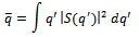
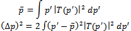
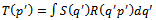
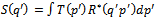
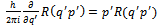
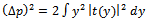
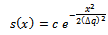
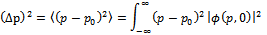
Heisenberg’s 1927 paper⁶ gives a proof of uncertainty principle, we discuss that later. However, his book⁷ of 1930 gives more details about the proof. In this proof he made two important assumptions: (A) he assumes that momentum and position are related by FT pair, and (B) he ignores the infinity assumption of FT theory.

The following proof is taken from the book: Heisenberg⁷ pages 15-19. In all integrals, Heisenberg assumes, the lower limit is -∞ and the upper limit is +∞. This is an important assumption, which goes against the finite space time law and the boundedness law. Therefore according to our definition of invalidity, this theory cannot be tested. The average value of the position q of an electron can be given by the probability amplitude S(q’) as:

Then is defined by

(2)

This can be called the uncertainty in the knowledge of the electron’s position. In the same way the momentum p and its uncertainty may be defined as

(3)

Here T(p’) is the probability amplitude of the electron’s momentum. After these definitions, Heisenberg makes his very crucial assumption. He claims that the two probability amplitudes are related by the equations

(4)

(5)

Observe that (4-5) are equivalent to an abstract Fourier Transform pair. He reveals the details within next few steps given below. This is a very unrealistic assumption on nature. There is no reason to believe, that nature will know our mathematics, and then obey the relation (4) and (5), connecting position and momentum.

He defines R(q’p’) as the matrix of the transformation from a Hilbert space, in which q is a diagonal matrix, to one in which p is diagonal. The matrix R(q’p’) satisfies the following equation

(6)

which is equivalent to the differential equation

(7)

Whose solution is given by

(8)

The details of (6-7) are given in the Appendix of the same book⁷ which uses functions and Schrodinger’s equation. Observe that (6-8) are equivalent statements, i.e., one can be derived from the other. Thus the form of R in (8) could have been assumed directly. In the next proof we show, that is what has been done.

Normalizing gives c the value . He claims, quite naturally that, the values of Δp and Δq are thus not independent. This is also obvious from his assumption of relating p and q via (4-5). To simplify further calculations, he introduces the following abbreviations:

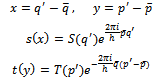Then equations (2) and (3) become

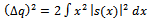(9)

(10)

while equations (4-5) become

(11)

(12)

The expressions (11) and (12) can be verified by direct substitution of definitions of x, y, t(y), s(x), and R in (4) and (5). Observe that (11-12) could have been directly assumed instead of (4-5), since they all are merely assumptions. There was no need to introduce the intermediate steps related to (4-8). In fact in the next proof of uncertainty principle given in next subsection we will see that we can jump from (3) directly to (11).

Now we can clearly see that (11) and (12) are classical infinite Fourier Transform pair, (10) represents the variations in time and (9) represents variations in spectrum. Thus the uncertainty principle is nothing but the product of time and bandwidth. We will talk more about the time bandwidth product later in another section.

Combining (9-11), the expression for may be transformed, giving

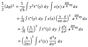Thus he writes, by using integration by parts, and noting that S(q’) is related to probability density function vanishing at two ends:

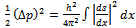(13)

Now the following expression

can be proved by rearranging

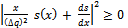(14)

Hence it follows from equations (9) and (13) that

Or

(15)

which was to be proved. The equality can be true in (15) only when the left side of (14) vanishes, i.e., when

or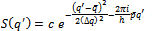

where c is an arbitrary constant. Thus Gaussian probability distribution causes the product to assume its minimum value.

In summary, Heisenberg assumed that momentum and wave functions are related by the Fourier transform pair (11) and (12). Then he defined the variances of the time and spectrum functions using (9) and (10). Then a simple algebraic manipulation proved the uncertainty relation (15). From (15) we see that uncertainty is the product of time and spectrum variances (bandwidth) of FT pair. It is clear from the above proof that there is no physical or experimental support behind the result (15), the uncertainty principle. It is a consequence of Fourier Transform which has its own assumptions as we will examine later. In particular, we will show that by removing infinity assumption we can remove the uncertainty.

4.2. Ohanian’s Method

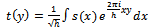
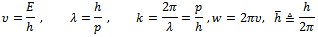
A relatively modern textbook by Ohanian⁸ gives the proof of uncertainty principle in the following way. This proof also makes the same two assumptions that Heisenberg did. Ohanian begins his chapter two, on page 21, with the following physical relations obtained from experiments and calculations

Then on page 22, Ohanian⁸ starts with four conceivable harmonic waves

Using some selection criteria he finally decides that from the list as the correct wave function describing a free particle. Then he finds the equation that this function must satisfy. He writes, it is easy to check that the second derivative of with respect to x and the first derivative with respect to time t are proportional, that is, we can write

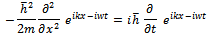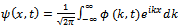
The above equation is a linear equation and therefore will be compatible with the superposition principle. Therefore any function that can be written as a superposition of a finite or infinite number of waves of the type will satisfy the differential equation

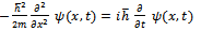(16)

The above (16) is the Schrodinger’s wave equation for the free particle. Then on page 32 Ohanian introduces the FT

(17)

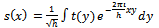
The function is called the amplitude in momentum space. This is where Ohanian makes the same assumption as Heisenberg did. He assumes position and momentum are related by inverse FT. There is no reason to believe that nature will obey this relation. This assumption is also not based on any experimental observations. On the other hand it is quite natural that a particle can have any momentum at any position. Also note that it introduces the infinity assumption in (17). Then he finds by substituting (17) in (16) giving

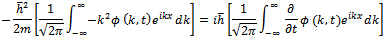Now comparing both sides the coefficients of we obtain the following differential equation

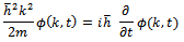Which has the solution given by (18); this way Ohanian gets a general expression (18) of momentum in the time dimension.

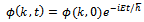(18)

where

Thus the general solution of the Schrodinger’s wave equation for a free particle can be written from (17) as

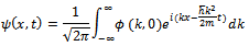The above solution can be written in terms of the momentum as in (19)

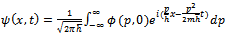(19)

Thus the last equation makes a direct connection of momentum and position via Fourier Transform. Therefore, as mentioned by Heisenberg, the two properties of the particle cannot be independent now. This will naturally dictate the uncertainty principle. If we assume something in some place then naturally consequence can be observed at another place.

Now on page 39 Ohanian⁸ introduces the Gaussian wave packet as momentum amplitude in the p dimension.

(20)

The advantage of choosing momentum as Gaussian function is that its inverse FT is also Gaussian. This helps to find the variances easily. Heisenberg had to compute the variances in a complicated way, Ohnaian skipped that complicated derivation. Ohanian then says, for a precise definition of the uncertainty of any quantity with a probability distribution, we will hereafter adopt the root-mean square (rms) deviation from the mean. Thus

Calculation of the integral using (20) gives the result

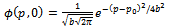
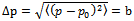Substituting the Gaussian momentum amplitude (20) into equation (19) we find the wave function

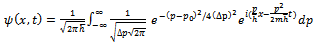(21)

From above we can derive the result

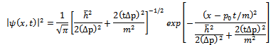From the last expression we see that the mean is and we can then find that the uncertainty in x is as given by

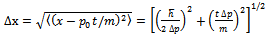(22)

From this (22) we see that at t=0 the uncertainty relation:

From (22) we see that for all other time for a given the value for increases because of t in (22), which then gives

We can see from this proof that the uncertainty principle can be proven without going through the higher level analysis that Heisenberg has given. Note that Heisenberg also uses the Schrodinger equation. It is clear from Ohanian’s proof also that there is no physics involved. It is all mathematical manipulation of FT theory.

Summarizing, Ohanian⁸ assumes that momentum and wave function are related by the infinite inverse FT in (17). He then gets a general expression (18) for the time dimension of momentum by using Schrodinger’s equation. Then he assumes a Gaussian function (20) for the momentum dimension. Finally the uncertainty result is obtained as the product of the variances from (20) and (21).

Thus we see that Ohanian’s proof is almost same as the Heisenberg’s proof, so far as assumptions are concerned. There is no physics involved here; it essentially tries to say that whatever happens in mathematics, will happen in nature also. The proof forgets that nature cannot make the two assumptions used in the derivations (a) infinity in FT and (b) the relation (17) that says momentum and position are related by the FT. It cannot be said that this uncertainty relation is derived from any experimental observation.

On the contrary, all experimental efforts to verify the principle will inevitably fail, because we cannot setup the assumptions used in the derivation. In particular, we cannot test it for infinite time as required by the theory of Fourier Transform. The theory is valid only under infinite time assumption. As we show later, if we replace the infinity by any finite value then there will be no uncertainty. Thus finite time approximation cannot be used to test the principle. Finite time will not be an approximation, it will be a dramatic change as we have mentioned.

4.3. Operator Theoretic Proof

This proof is based on the operator theoretic approach and follows closely the book⁹. It shows that the uncertainty principle is a property of Hermitian operators on Hilbert space. In our analysis we may consider measurable functions along with Lebesgue integrations.

However, we point out that in engineering we never see even piecewise continuous functions with discrete jumps. Thus non-continuous measurable functions are non-existent in nature. If we put an oscilloscope probe on any pin of a digital microprocessor you will always see a continuous function. Thus piecewise continuous functions are nonexistent even in digital systems. Moreover we are not thinking about infinity, thus real life, in mathematical sense, is not at all abstract. Thus it is difficult to believe that nature will obey our manmade abstract mathematics, which is so full of assumptions.

This derivation makes three assumptions. (A) It uses a Hilbert space, which is a linear vector space. As we have described before, because of the boundedness law there is no linear space in nature. (B) It assumes infinity in its definition of inner product. We know that infinity violates the finite time law. (C) It assumes isolated environment violating the simultaneity law. Thus we see that this theory cannot be tested also, because of the infinity assumption, if not for any one of the other assumptions. In the following, first we show the proof, and then we discuss their assumptions.

Let V be a complex Hilbert space, let and be any two complex valued functions in V, let the inner product in V be denoted by

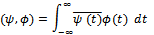For convenience we note the following properties of complex inner product:

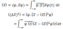
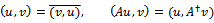Let X be a linear operator mapping V into V. Then we define the mean and variance of in the following way, with respect to a given normalized vector .

We present the following lemma⁹, called the Schwartz inequality taken from page 14; the proof is given in a later section.

Lemma Let and be two arbitrary vectors. Then

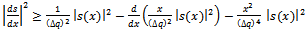
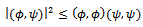The proof of uncertainty principle starts with the following lemma⁹ on page 119.

Lemma Let O₁ and O₂ be two Hermitian operators. Then

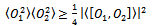(23)

The mean values are computed using any normalized vector .

Proof Let us apply the Schwartz inequality to vectors and. Because O₁ and O₂ are Hermitian, one has

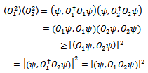(24)

Letting

One sees that and so that

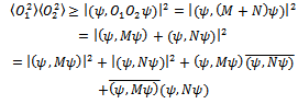(25)

The third and fourth terms in the last inequality (25) cancel each other. The first and second terms being nonnegative, one finds that

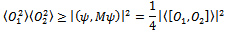End of proof.

Let us now apply the lemma to the case where

One has

Thus one gets

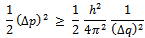
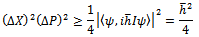From which Heisenberg’s inequality immediately follows.

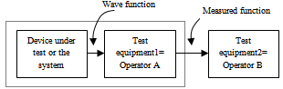Figure 2. Operators cannot be cascaded

The proof essentially computes the product of two variances using Schwartz inequality. The crucial step is expression (24) which is derived from Schwartz inequality. To understand why (24) happened we have to understand inner steps of Schwartz inequality, which we discuss in another section.

Hopefully the reader noticed that the proof is completely mathematical in description and does not have any connections with physics or quantum mechanical particles or nature. So, essentially this proof claims that whatever happens in mathematics, will happen in nature also. Is that how we really think? How did we get so much confidence on our manmade mathematics? What were we thinking about all the assumptions behind our mathematics?

It cannot be said that this derivation is a consequence of any experimental observation. On the contrary, it has so many assumptions that it can never be tested by any engineering experiment. As mentioned, the proof assumes: linearity, infinity, and isolated environment. It will never be possible to setup an environment that will satisfy all the assumptions; because nature does not and cannot allow such assumptions. As we have mentioned operators, Hilbert spaces, Schwartz inequality, inner product, all violate the boundedness, finite time, and simultaneity laws. Thus operator theory does not recognize the complexity of nature.

From (23) we see that if the operators commute then there will be no uncertainty. But operators will never commute, because the second operator is not working on the system. Repeating operators, like in (24), is a violation of engineering practice. It is an assumption.

Figure 2 dictates the block diagram for testing the uncertainty principle based on the operator theoretic proof. In Figure 2, the device under test (DUT) is the system which is generating the state vectors or wave functions. All operators are like experiments or like test equipments that are used to test the DUT. Operators are designed to work only on DUT. In the figure operator A is denoted by an experiment or test equipment1 that tests the output signals from DUT. Input to operator A is the wave function from the DUT and its output is a measurement function. We can see that cascading means operator B is not working on the DUT or the wave function, but on the measurement function. Measurement function is not same as the wave function. Measurement function is not generated by the DUT; it is generated by the test equipment1.

The two input signals are different, they come from different environments, and they cannot be comparable. The cascading theory violates the simultaneity law. Once an operator is used on a wave function its output cannot be a wave function again. Wave function does not remain a wave function when it is processed and taken out of its environment. In the absence of the simultaneity environment, a wave function loses its characteristics. Nature is immensely complex, anything taken out of environment, behaves completely differently. Thus cascading is equivalent to the assumption of isolated environment, as in Newton’s first law, which we know cannot work.

The characteristics of an object significantly change when it is taken out of its environment. When I am outside my home, I am a completely different person. Earth taken out of its orbit will not remain as earth. Same is true for the operator outputs. Thus the concept of commutation is not meaningful in engineering. Cascading operators is an assumption; it is not meaningful for engineering test of a theory. Figure 2 becomes an invalid test setup for testing uncertainty principle. Figure 2 shows that the operator theoretic proof is inconsistent with nature.

The proof is also invalid for many other assumptions we have mentioned, like infinite space time assumptions. We have discussed them in other places. In this section we elaborated the cascading requirement only, which violates the simultaneity law. Thus the operator theory cannot be tested, and according to our definition of invalidity, the operator theory cannot work.

5. Schwartz Inequality

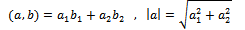
The Schwartz inequality is a very simple concept of mathematics. Here we present the definition, theorem, and its proof from a standard textbook like Eideman¹⁰. We need the details to see that the root cause of the uncertainty principle is hidden behind this theorem. If we take two 2-dimensional vectors, a and b, then we know that their dot product or inner product is given by

(26)

where is the angle between the two vectors; means the magnitude or the length of the vector. Since cosθ is always less than or equal to 1, we can write the Schwartz inequality as in

(27)

We see that the above is a trivial relation. Take a = 4, and b=2, the relation will hold. It will be always true, like 2 < 4 or a < (a+1). Thus we must be careful then how we use them. We should not assign any function to a and any other function to b and compare those using (27). It will not be meaningful, for example, to assign voltage to a, and price of apples to b in (27).

If we define the inner product and magnitude in the following way

Then we can see the Schwartz inequality of real numbers as

It is clear that the above is valid for n-dimensional vectors. In case of n-dimensional vectors, cosθ can be defined as

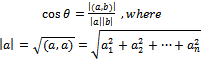(28)

Along the same natural way, we can extend the sum to integral to write the Schwartz inequality for integrals as

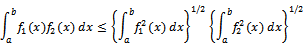Clearly the integral Schwartz inequality will still remain valid for infinite limits for the integrals in the last expression under the assumption of appropriate integrability conditions.

Theorem: Let u and v be arbitrary members of an inner product space V. Then the Schwartz inequality is given by

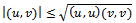Proof: If v=0 then clearly theorem is satisfied. Assume then that . For an arbitrary scalar ,

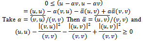Or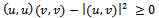

From which the assertion follows. Note that is same as cos as defined by (28). A pictorial view of (26) will show why the expression is correct.

From figure 3 we can see the real meaning of the Schwartz inequality. Clearly the product of the magnitude or the length of the two vectors a and b is bigger than the product of b and c. The product of b and c is whereas the product of a and b is simply. This is a purely mathematical property; it requires complete isolation from any other physical requirements. It is a manmade theory lives in isolation from nature. A manmade theory cannot be a law of nature. All laws of nature must be experimentally observed by using engineering experiments.

Figure 3. Schwartz inequality for vectors

Application of this dot product to any two vectors is meaningful only when the vectors belong to same class of objects. If vector a represents apples and vector b represents oranges, then clearly the dot product will not be meaningful; the angle θ will also not be meaningful. Since every operator produces a function which is different from the one produced by another operator, these two output functions of operators cannot be compared, they belong to two different object classes. Two measurements, like and, taken by two different operators on the same vector are two different objects, like apples and oranges. Therefore applying dot products on them are not meaningful. As mentioned, an operator represents an experiment on objects of nature. Two operators represent two different experiments. Their use in (24) or in Figure 3 is inconsistent with engineering concepts of an experiment.

To illustrate the incompatibility of the operator outputs, the following example may be better. Suppose we take a cat described by four different properties and represent it using a vector [c₁, c₂, c₃, c₄], similarly we a take a dog described by another five different properties represented by[d₁, d₂, d₃, d₄, d₅]. These two vectors represent simultaneous environments of cats and dogs respectively. Let us now use an operator C that converts the cat vector in to a two dimensional vector of numbers, and similarly we take another operator D and convert the dog vector to another two dimensional vector. (Note that C and D are not entirely meaningless. We use them in our manmade society. In economics, we convert every human being to a money value.) Even though the resulting vectors are of same dimensions we cannot still take their inner products, because by the equivalence principle as described later, they are different objects. The properties of cats and dogs are embedded in the two vectors, making them in eligible for dot products. Thus the application of Swartz inequality to derive uncertainty principle is not meaningful.

Algebra makes a very fundamental assumption: all variables belong to the same class, like real numbers. In nature, things are never same. We always have apples and oranges. Even two apples are different. Just like we cannot add two apples and three oranges to give five apples or five oranges, in the same way we cannot add five apples also, because all five apples are different. In reality, even algebra has very limited applications in nature. We must remain vigilant about the applications and the assumptions of mathematics.

No variable in nature is isolated; they are all connected by simultaneity law with many other things in its environment. Thus each variable is unique. No two variables can be compared. The core assumption in algebra is isolation of variables, which is invalid in nature. Nature obeys the simultaneity law. We can only compare output of same operators but not two different operators. We cannot compare apples and oranges. The two functions and used in (24) are like apples and oranges, when are all objects of nature. They are not merely mathematical entities.

6. Time Bandwidth Product

In this section we give another proof of uncertainty principle. We first show that the well known dimensionality theorem is same as uncertainty principle. This proof will show that the uncertainty principle violates a fundamental property of mathematics – all continuous functions over finite interval are infinite dimensional. Eventually this analysis will then show how we can eliminate the uncertainty. According to Heisenberg⁶ - “If there existed experiments which allowed simultaneously a sharper determination of p and q than equation (1) [Uncertainty relation] permits, then quantum mechanics would be impossible”. However, it is believed that QM is not about the theories; it is about the experimental evidences and accumulated knowledge on the results we have on the subject. No theories of any subject can be correct, because of the baggage of assumptions they carry, since we know nature does not and cannot make any assumptions.

6.1. Fourier Transform

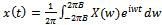
The Fourier Transform (FT) has become a fundamental tool for many branches of science and engineering; quantum mechanics, as we have just seen, is no exception. The FT pair is defined as:

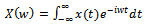(29)

(30)

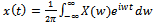
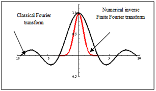
Equation (29) gives the FT, X(w), of the time function, . Expression (30) gives the Inverse FT from the spectrum function, , and produces the time function, x(t). In a previous section we have given two proofs that show that uncertainty principle is derived from the FT theory. In this section we analyse the FT in more details to find the root cause of this uncertainty.

Observe that both integrals have infinity as limits. One way to examine this infinity requirement of FT is to visualize the example of the delta function. Its FT is 1 for all w. That means all cosine functions that create the delta function have unit amplitude and zero phase. If you draw some of these cosine functions, see Priemer¹¹ in pages 178-179, you will find that the functions are adding up to create the pulse and becoming zero at all other places. This example shows that all cosine functions must be defined over all time, and the same must be true for the delta function also. That is, the delta function must exist as zero for the entire real line except the place where it is non-zero.

Consider the time function shown in Figure 4 and the corresponding Fourier transformed spectrum function shown in Figure 5. The graph in Figure 5 was obtained using expression (29). Both functions must be defined and must exist for the entire x-axis as required by the FT theory. The width of the distribution in spectrum Δw is 4π/ΔT and the width Δt = ΔT of the distribution in time function can be regarded as uncertainties. The product of these two uncertainties show that

(31)

The quantum mechanics textbook by Ohanian⁸ page 35, says (31) “is an instance of Heisenberg’s uncertainty relation”. The same idea is described in the engineering book, Soliman¹² pages 214-216, and has the section heading “The Uncertainty Principle”.

The expression (31) is known as Time-Bandwidth product, and also as Dimensionality theorem in the field of digital communication engineering, see Couch¹³ page 93. Clearly (31) is a characteristics of Fourier transform pair as we have seen in the two proofs given above. Since the spectrum function is derived from the time function, the two functions are related, and (31) represents one such relation. More details of such relationship are described in a later section.

All continuous functions can be considered as infinite dimensional vectors. This fact is quite well known in quantum mechanics community; see for example Chapter 4 of Miller¹⁴. However, for completeness we present the following theorem, without proof, from Das¹⁵, over finite duration intervals.

Let f(t) be a continuous time function defined over L₂[a,b], the space of square integrable continuous functions over[a,b]. For engineering we do not need measurability and Lebesgue integrability. Assume that we divide the finite time interval[a,b] into n ≥ 1 equal parts using equally spaced points . Where and. Use the following notations to represent the t-subintervals

then define the characteristic functions:

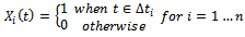and the simple functions:

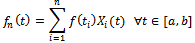Theorem 1

The above theorem, Das¹⁵, essentially says that the sequence of step functions, with step height defined by the sample values, converges to the original function. These samples, collected as a column vector represent the infinite dimensional vector for the function. Thus given any accuracy limit, a step function can be generated that will represent the function with that accuracy. The theorem says that this conclusion is valid for any finite interval.

Figure 4. Time function

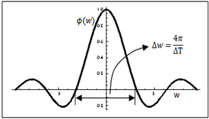Figure 5. Spectrum function

6.2. Dimensionality Theorem

The dimensionality theorem is stated in Couch¹³ page 93, as: “When BT is large, a real waveform may be completely specified by N=2BT independent pieces of information that will describe the waveform over a T interval. N is said to be the number of dimensions required to specify the waveform, and B is the absolute bandwidth of the waveform”.

Comparing with equation (31) we can see that Δt = T and Δw = 2B. Thus the dimensionality theorem is same as uncertainty principle. We show that the dimensionality theorem is derived from FT and requires infinity assumption. Thus we can say, dimensionality theorem = time bandwidth product = uncertainty principle. They are all equivalent to FT and are derived from it, in different branches of science and engineering by different people.

Clearly this dimensionality theorem violates the property described by Theorem 1, that a function is infinite dimensional, even over finite interval. For thedimensionality theorem says that N is a finite number, and N number of samples completely specifies a function. This happens because the dimensionality theorem assumes that T and B both represent finite intervals, which goes against the requirements of the FT pair described by (29) and (30).

In order to prove the dimensionality theorem we need to use the Nyquist Sampling Theorem. This is a very well know theorem in the digital signal processing field but may not be known to quantum mechanics community. This theorem is stated in the following way, Couch¹³ page 89, we skip its proof.

6.3. Nyquist Sampling Theorem

“The minimum sample rate allowed to reconstruct a band limited waveform without error is given by f_s = 2B”. Here B is bandwidth and f_s is the sampling rate also known as the Nyquist rate.

The following proof of dimensionality theorem is based on Shannon¹⁶. In case of a band limited waveform, that is, a waveform whose spectrum is zero outside a finite bandwidth[-B,+B], the expression for inverse Fourier transform (30) can be rewritten as

(32)

In (32) t goes from to , because x(t) comes from (29), the FT. Replacing time t by Nyquist sampling interval we get

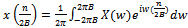(33)

Recognize that the left hand side of (33) is the Fourier series expansion coefficients for X(w). In (32) t goes from to and therefore it is same for n in (33). Thus the function x(t) can be “completely specified”, as stated in the dimensionality theorem, once we get all the coefficients from (33), construct the X(w) from them using the Fourier series, and then use that known X(w) to reconstruct x(t) using (32). Observe that this process requires infinite number of samples using all values of n in (33). Thus function x(t) must be defined for all t to make the process work. A Fourier series requires infinite number of coefficients.

Thus the total number of samples required to recover the signal x(t) for very large value of T is given by

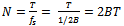(34)

We see that the dimensionality theorem (34) is derived from FT, and requires infinite duration assumption for x(t).

However (34) cannot be correct, because it violates our Theorem 1, which says that a function is infinite dimensional even over a finite interval. Thus if we use formula (34) we will always get an error with a lower bound in representing the time function x(t). That is, any accuracy we want cannot be achieved using N samples. The expression (34) is same as the uncertainty principle of quantum mechanics as described in (31). Here we see that uncertainty principle violates the infinite dimensionality property of finite duration signals. Real problem here is that we are trying to find properties of finite duration signals using properties of infinite time theory. In reality all functions, finite or infinite durations, are infinite dimensional. Uncertainty principle contradicts that theory.

This leads to the idea of infinite limit assumption of the FT theory. According to the finite time law, infinity is invalid in nature. Therefore anything that considers infinity, like FT theory, will also be invalid. The use of such results will cause inconsistency and contradiction. In the next section we replace infinite limits in the FT definition by finite limits and show that we can remove uncertainty.

Figure 6. Different spectrums for same pulse

7. Finite Fourier Transform

We now show that if we eliminate the infinity assumptions from Fourier transform expressions in (29) and (30) then we can overcome this lower bound error limit from the uncertainty principle.

We use the principles behind the numerical inversion of Laplace transform method as described in Bellman¹⁷. Let X(w) be the unknown band limited Fourier transform, defined over[-B,+B]. Let the measurement window for the function x(t) be[0,T], where T is finite and not necessarily a large number. Divide the frequency interval 2B into K smaller equal sub-intervals of width ∆w with equally spaced points {w_j} and assume that {X(w_j)} is constant but unknown over that j-th interval. Then we can express the integration in (32) approximately as:

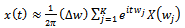(35)

The right hand side of (35) is a linear equation in {X(w_j)}, which are unknown. Now we can also divide the interval[0,T] into K equal parts with equally spaced points {t_j} and let the corresponding known sample values be {x(t_j)}. Then if we repeat the expression (35) for each sample point t_j we get K simultaneous equations in the K unknown variables {X(w_j)} as given by the equivalent expression (36).

(36)

The equations in the matrix vector expression (36) are independent because exponential functions in (36) are independent. Therefore we can solve (36) for {X(w_j)}. Theorem 1 ensures that the sets {X(w_j)} and {x(t_j)} can be selected to achieve any level of accuracy requirements in (32) for either x(t) or X(w). For convenience we assume that the number of terms K in (36) is equal to K = Tkf_s =2kBT. Here f_s is the Nyquist sample rate and k > 1. We state the following theorem from Das¹⁵, which essentially is a modification of the Nyquist’s sampling theorem.

Theorem 2

Let x(t) be a band limited function with bandwidth restricted to[-B,+B] and available over the finite measurement window[0,T]. Then given any accuracy estimate ε there exists k>1 such that 2kBT equally spaced samples of x(t) over[0,T] along with their sinc functions, will completely specify the function x(t) for all t in[0,T] at the given accuracy ε.

Theorem 2 says that by increasing the sample rate we can achieve any accuracy in describing the spectrum function and the time function. The sampling factor k is a multiple of the Nyquist rate. In industry it is quite common to use 4 or 5 times the Nyquist rate to get correct results. In Das¹⁵ a numerical example is given to show how k affects the accuracy in recovering the time functions. Thus this result is quite well known in the industry, we have just added a theoretical proof of this common practice.

In Figure 6 we show, using a numerical example, how the unit pulse of Figure 3 with ΔT=2 can be reconstructed using (36) for various values of bandwidth. The red graph is derived for a bandwidth of π, and K = 20 as number of samples. The black graph represents the classical FT of the pulse in Figure 3. Figure 6 shows how a narrow bandwidth red spectrum can generate the same time function when we eliminate infinity assumption. A larger bandwidth spectrum could have been used also, but with a different sample rate to create the same pulse. We call method (36) as numerical inverse finite Fourier transform, NIFFT.

It is clear from Figure 6 that the uncertainty relation (31) does not hold if we use (36). Expression (36) gives many solutions for spectrum for the same time function and depends on values of K and bandwidth. By eliminating infinity, the formula (36) brings two additional degrees of freedom, a choice of band width and a sample rate. These two degrees of freedom make (36) an independent method of constructing waveforms. The rectangular pulse generated from the red spectrum is same as shown in Figure 4. 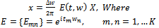The Mathematica software tool was used for the numerical inversion algorithm (36).

8. Discussions

In this section we point out certain views that may indicate how the idea of uncertainty principle may have originated.

8.1. The Origin

The origin of the uncertainty principle seems to have emerged from the Heisenberg’s 1927 paper. We quote a portion of a paragraph from that paper, Heisenberg⁶ pages 64-65, which is still mentioned in present textbooks, and taught in class room lectures on YouTube videos. This is also another proof of uncertainty principle.

“However, in principle one can build, say, a γ-ray microscope and with it carry out the determination of position with as much accuracy as one wants. In this measurement there is an important feature, the Compton effect. Every observation of scattered light coming from the electron presupposes a photoelectric effect (in the eye, on the photographic plate, in the photocell) and can therefore also be so interpreted that a light quantum hits the electron, is reflected or scattered, and then, once again bent by the lens of the microscope, produces the photo effect. At the instant when position is determined-therefore, at the moment when the photon is scattered by the electron-the electron undergoes a discontinuous change in momentum. This change is greater the smaller the wavelength of the light employed-that is, more exact the determination of the position. At the instant at which the position of the electron is known, its momentum can therefore be known up to magnitudes which correspond to that discontinuous change. Thus more precisely the position is determined, the less precisely the momentum is known, and conversely. In this circumstance we see a direct physical interpretation of the equation

Let q₁ be the precision with which the value q is known (q₁ is, say the mean error of q), therefore here the wave length of the light. Let p₁ be the precision with which the value of p is determinable; that is, here, the discontinuous change of p in the Compton effect. Then according to the elementary laws of the Compton effect p₁ and q₁ stand in relation p₁ q₁ ~ h.”

It is not known, how much of engineering technology existed in 1927 and how much familiarity a theoretical physicist like Heisenberg had about that engineering. Clearly in modern times this will not be the design of an experiment by any stretch of mind of any system engineer. Two unknowns cannot be found out by one measurement; this will produce one equation in two unknowns. At least two equations will be necessary to solve for both p and q variables. Heisenberg seems to believe that only one measurement will give values for both p and q. This is an assumption he used unconsciously. In reality, a significantly large volume of dynamic data should be collected, for a long period, both before and after hitting the electron, all simultaneously, and then eliminate all unknowns by least square curve fitting algorithm of dynamical systems, something like Kalman Filtering.

It is almost unbelievable that how much accuracy we can achieve using modern technology and with such simultaneous measurements. Simultaneity is a law of nature, more we encompass it better results we get. GPS satellites are about 20,000 km above earth. Yet we can measure distances on the surface of earth at the accuracy of sub-millimeter level, see Hughes¹⁸, in geodetic survey, by measuring the satellite distances. In one sense then we can measure a distance of 20,000 km at the accuracy of sub-millimeter. This approach uses only non-military GPS signals. So we can think, how accurate the results can be, with the exact military signals from new generation of GPS satellites and receivers. Thus at this modern time, in retrospect, it is difficult to understand why Heisenberg thought about such an experiment involving one measurement to identify two variables.

8.2. Equivalence Principle

It is very fundamental to recognize that a function can be represented in many equivalent ways. For example (a) It can be described by providing a table of values of x coordinates at fixed intervals and corresponding values of y coordinates, as numerical data; (b) The above table of data can be interpolated and then represented by a smooth graph in the x-y plane; (c) It is also possible to represent the same graph using an algebraic equation of y as a function of x; like y= 3x+x²; (d) It can be represented by a combination of sinusoidal or exponential functions, like Fourier or Taylor series; (e) derivatives can be taken on this algebraic function, and a differential equation, like Schrodinger equation, can be produced to represent the same data; (f) we can perform an integral transform of the algebraic expression to create something like Fourier transform to represent the graph; (g) It is also possible to describe the data as a function in inner product space with operators, like integral or differential operators, or even abstract operators like Hermitian infinite matrices to describe the data.

It is clear that all of the above representations of the numeric data in (a), are equivalent. This various representation methods may be called equivalence principle. In fact Ohanian⁸ on page 33 admits that – “The free-particle Schrodinger equation does not produce any solutions except those that can be directly constructed by superposition – the equation gives us nothing new”. Any information derived from any one of the above items can be derived from all other representations. They only enhance the conveniences.

A better and sophisticated look at the numerical data in (a) will definitely allow us to visualize the graph. Similarly we may be able to visualize the spectrum from the graphical representation (b) of the numeric data. The information content of the time function and its spectrum is same, because one can be derived from the other. Thus Fourier Transform cannot give any new information that is not present in the numeric data in (a) or the graphical content in (b). An experienced eye will be able to observe the harmonic contents of FT in the graph, although not numerical values. It will be possible to get the fine characteristics of the data from any one of the above equivalent representations.

Thus there is no reason to believe, as is done in quantum mechanics, see Ohanian⁸ pages 32-36, that if the time function represents the position of the particle then the corresponding spectrum function will represent the momentum. Position and momentum are two independent variables of a dynamical system. It was very unfortunate that Heisenberg linked them via the FT pair (14-15). FT pair cannot give any new information as explained in above. As a consequence of this FT property, Heisenberg has to introduce uncertainty principle causing more confusion. This position-momentum relationship via FT does not satisfy engineering or physical intuitions. Both time and spectrum functions are different representations of same thing; on the other hand both position and momentum are independent properties of a particle. The uncertainty principle (31) is thus a mathematical consequence of equivalence principle.

9. Conclusions

We have shown that the uncertainty principle is a property of the Fourier transform theory. In addition, the Fourier transform uses infinity as its assumption; and elimination of infinity assumption removes this uncertainty. The paper also derived that uncertainty principle violates a fundamental property of mathematics – all continuous functions over finite interval are infinite dimensional. We have pointed out many laws of nature that engineering implements, but math and science ignores them. These laws cannot allow cascading of Hermitian operators, and use of Schwartz inequality to physical variables. It is a fact that nature and engineering cannot and do not make any assumption, but math and science do. Therefore, no math and science theories can be tested by any engineering experiment, because experiments cannot implement the assumptions required by all theories.

ACKNOWLEDHEMENTS

At many stages during the development of this research many people helped in many different ways. The author is deeply indebted to Professor Nirode Mohanty, Professor Avatar Singh for their contributions at the early stages of this research. Dr. Nibir Datta, a friend and colleague, has helped in formulating the ideas on the inability of experiments to verify the theories.