Bello R. , Agbaoye R. Olamide
Department of Physics, Federal University of Agriculture, Abeokuta, Nigeria
Correspondence to: Bello R. , Department of Physics, Federal University of Agriculture, Abeokuta, Nigeria.
| Email: |  |
Copyright © 2012 Scientific & Academic Publishing. All Rights Reserved.
Abstract
In spite of the importance of the temperature of the ground, only little model has been established for the earth temperature at 5cm and 10cm below the ground surface. This piece of research work is useful in generating the temperature of the earth at these depths for many years to come as long as other environmental factors are available for these years. The environmental factors used in this work, were recorded and obtained from Nigeria Meteorological service (NIMET), SPSS was used for the data analysis and the outputs was discussed in detail to extract the equations of the earth temperature at both depths. MATLAB programming language was used to generate the computed values of the earth temperature from the equations obtained to test its validity. The observed and computed data were compared and subjected to statistical test for validation. The test showed no significant difference between the observed and the computed data. Information on ground temperature is important for many construction projects, installation of underground pipes and cables, survival and nutrient distribution in plant.
Keywords:
Temperature, MATLAB, Modeling, SPSS, Environmental Factors
Cite this paper: Bello R. , Agbaoye R. Olamide , Modeling of Ground Temperature as a Function of Some Environmental Factors, International Journal of Theoretical and Mathematical Physics, Vol. 3 No. 1, 2013, pp. 36-46. doi: 10.5923/j.ijtmp.20130301.05.
1. Introduction
Geothermal energy is made up from the heat of earth. Billions of years ago, mixture of dust and gases resulted into geothermal energy. At the core of earth temperature is approximately 9,000 F and its heat has outward flow, which is transferred in all the adjoining rock layers. Figure (1) shows increase in earth temperature with depth. Since the early 20th century, Earth's mean surface temperature has increased by about 0.8 °C (1.4 °F), with about two-thirds of the increase occurring since 1980. | Figure 1. Earth Temperature as a Function of Depth |
Modeling is a core research tool that requires the use of methods such as differential equations, probability, statistics,linear programming, and game theory or other forms to predict, analyze and interpret theories, with respect to some initial condition[1].Predictive model forecast the likelihood of future events or condition based on quantitative data or information from the past[2]. A number of predictors influence the result of a predictive model, which in some cases is referred to as the independent variables. To create a predictive model, data or information of relevant predictors are collected, sorted if the need arise and a mathematical expression is created using statistical analysis techniques. The statistical analysis is interpreted to derive a model; the validity of the model is tested by calculating the value of the dependent variables as a function of the independent variables of the collected data.
2. Matrix Laboratory (MATLAB)
MATLAB is a high performance language for technical computing, it integrate computation, visualization, graphical command representation and programming environment[3], MATLAB is a vital tool in research and learning, several built-in tools for solving various computational, analysis, programming problems and lots more, are embedded in matlab interactive application interface. MATLAB is popularly known as an artificial intelligence that was written originally to grant access to matrix software that was developed by LINPACK (linear software package) and EISPACK (Eigen system package) projects.Matlab is an interactive system whose basic data element is an array that does not require dimensioning[4]; it has built in packages and routines that enable it to perform variety of useful computation, graphical command, and immediate visualization of result. Being an object oriented programming language with built-in editing and debugging tools had made it indispensible compare to other conventional programming language like C, FORTRAN, and PASCAL programming languages. Some of its applications are collected into packages such as Toolbox, Builder, Simulink Design, Embedded integrated design environment (IDE), target support package etc. The toolbox package contain application like aerospace, bio-infometric, control system, financial, mapping, curve fitting, fuzzy logic, and other science and engineering tools.
3. Computer Programming
A computer is an intelligent and versatile electromechanical device that accept, process, sort, stores and output data at high speed according to the programmed instructions. A computer cannot posses all these attributes without being commanded to do so, this command can be termed as codes or programs. Programming is an act or mode of communicating with the mechanical and electronic component of a computer through commands, raw coding, generated coding or processed coding called software. Examples of programming languages are FORTRAN (Formula translator), Pascal, Visual Basic, C, COBOL (Common business oriented language), Java, MATLAB , the simple language a computer can understand and interpret conveniently and directly is the machine language, the combination of the digit 0 and 1[5]. Programs written in machine language is tedious, prone to mistakes and difficult to debug, this lead to interacting with the computer using assembly language which require the use of mnemonics, an alphabetic abbreviation such as ADD, MULT etc. assembly language is first converted to machine language before it can communicate with the computer. High-level programming is developed to make programming less tedious, it is a huge improvement over the earlier programming languages[6], codes are written in near English language requiring either a compiler or an interpreter, which are programs, used to convert the near English high-level language into machine code of zero(s) and 1(s). An interpreter convert the codes a row after the other, while a compiler convert all the codes at once before running the program. High level programming can either be procedural oriented, which focus on the major task the program needs to perform, here the programmer must instruct the computer every step from the start to the completion. The programmer do not just inform the computer the appropriate code but the correct sequence or arrangement of the instruction is also required, examples are COBOL, BASIC, C., or an object oriented programming languagein which program are viewed instead as a collection of data objects that exhibit particular behavoir.
4. Regression Equation for N Amount of Variables
Regression equation is the mathematical expression of the relationship that exist between two or more variables as deducted from the line of best fit drawn on the scatter diagram. The least square regression provides a technique for estimating the equation of a line of best fit, this line is called the regression line[7]. Consider the relationship between two variables, y the dependent variable and x the independent variable.The steps required to derive the regression equation for 2 variables is stated by[7]. These steps can also be used to derive regression equation for n variabled as follow: | (1) |
Equation (1) is the equation of a straight line of best fit of two variables x and yWhere B0 is the intercept. B1 Is the regression coefficient for variable x | (2) |
For each observation of y, y is represented by equation (2).Where ej is reffered to as the error function.The error function is responsible for the difference between the value of y as deduced from the graph and the value of theoretical value of y.For n number of variables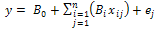 | (3) |
For n amount of variables and the amount of daysi Is used as a notation that identify the iteration of variablesj represent the number representation of the dayB0 Is the intercept in equation (3)B1, B2………………….. Bn Is termed as the regression coefficients x1,x2,…xn is termed as the number of the independent variablesyj Is the value of y for the jth day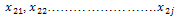 is variable x2 with jth number of dayFrom equation (3),
 ej Is the error factor that is responsible for the inconsistency between the computed data and the collected data, our prediction is better if our error function is insignificant.Making ej the subject of the formula in equation (3).
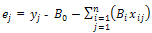 | (4) |
To minimize the effect of the error term we compute the Sum of Square Error (SSE)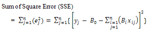 | (5) |
To remove the error term  | (6) |
 | (7) |
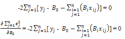
From equation (6), , differentiating the Sum of Square errror with respect to B0 we get
 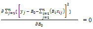 | (8) |
 | (9) |
Dividing through by 2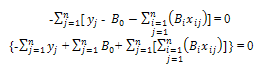 | (10) |
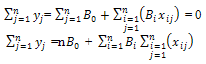 | (11) |
Recall that  from equation (7)
 | (12) |
Since Bi is a constant then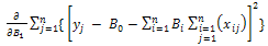 Since
Since  Differentiating the Sum of Square, error with respect to
 | (13) |
Dividing all through by 2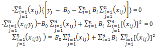 | (14) |
Rearranging and solving simultaneously by elimination method equations (11) and (14)By multiplying equation (11) by  and multiplying equation (14) by n
 | (15) |
Equation (15) is written as | (15b) |
 | (16) |
Subtracting equation (15b) from equation (16) gives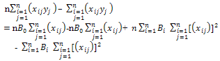 Collecting like terms and re-arranging
 Making
  the subject of the formular
 | (17) |
From equation (11)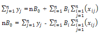 Making B0 the subject of the formula
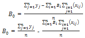 | (18) |
 | (19) |
 | (20) |
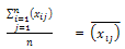
 Is the mean of the data values for the dependent variable for an ungrouped data?
 Is the mean of the data values for the independent variables of an ungrouped data for the jth day
 | (21) |
Recall that the regression equation for 2 variables is +  from equation (2).
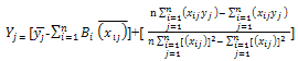 | (22) |
Therefore the regression equation for n variables is equation (22).Because of the complexity of this manual computation and the fact that any little inherent error will result in gigantic amount of accumulated error, it is necessary to introduce a statistical software, statistical package for social science that will reduce the error function and make our model fit for use.
5. Statistical Package for Social Science (SPSS)
SPSS is a statistical application that is used in data analysis across disciplines, it has ability to compute graphical representation, tabulation and presentation of data, its simplicity, error reduction and ability to produce output at run-time make it suitable for modeling mathematical expression for systems. It analyzes data through regression, correlation, mean, standard deviation and other statistical computation.Data input can be through the spreadsheet-like data editor or importing our data from database like excel, or other data acquisition software, with consideration on the syntax for naming variables on SPSS[8], then the data is analyzed by manipulating buttons on the menu bar. Using the SPSS to analyse the data in appendix (1) gives tables 1 to 7.
5.1. Analysis of Results
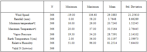
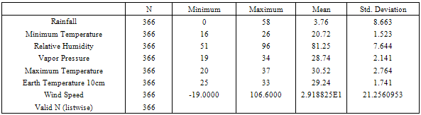
The following results are inferred from the SPSS analysis.Table 1. Descriptive Statistics (Earth Temperature 5cm)
 |
| |
|
Table 2. Descriptive Statistics (Earth Temperature 10cm)
 |
| |
|
Tables 1 and 2 show the descriptive statistics, which indicate the mean, standard deviation, minimum and maximum values of all independent variables for earth temperature 5cm and 10cm respectively. | Table 3. Model summary (Earth Temperature 5cm) |
| | Model | R | R Square | Adjusted R Square | Std. Error of the Estimate | | 1 | 0.775a | 0.601 | 0.595 | 1.65541 |
|
|
a. Predictors: (Constant), Wind Speed, Rainfall(mm), Minimum Temperature, Relative Humidity, Vapor Pressure, Maximum Temperature ℃| Table 4. Model Summary (Earth temperature 10cm ) |
| | Model | R | R Square | Adjusted R Square | Std. Error of the Estimate | | 1 | 0.915a | 0.837 | 0.835 | 0.708 |
|
|
The modal summary on table 3 and 4 shows the disparities that exist in the data value of the dependent variables. The coefficient of correlation (R) explains how sparsely located, the dependent variable data value is around the regression line. The coefficient of determination (R squared) measures the proportion of the total variation in the values of the dependent variable (Y) that can be explain or accounted for by variation in the independent variable (X), the value of R and R-squared is of the range of -1 and 1, (R- squared) explain how the data value of the dependent variable is scattered on the regression line. R-squared value shows the number of data point that is plotted on the regression line. In Table 4.3 the coefficient of correlation R = 0.775 shows that the plotted points are not too scattered apart, the coefficient of determination R-squared = 0.601, the R-squared value interpretation explains that the regression line of best fit passes through 60.1% of the points on the graph, this is a good fit for the regression equation at 5cm. In table 4.4 the coefficient of correlation R = 0.915, explains how sparsely located the dependent variable data value is around the regression line, the coefficient of determination R squared = 0.837 indicate that the data value of the depended variable is scattered on the regression line. However, the regression line passes through 83.7% of the points on the graph; this is a measure of how satisfactory our equation looks like. Table 5. Correlation (Earth Temperature 5cm)
 |
| |
|
Table 6. Correlation (Earth Temperature 10cm)
 |
| |
|
The correlation table, Table 5 shows the relationship that exists between all these variables by comparing them with one another.Rainfall has a weak correlation with minimum temperature and vapor pressure although the relationship is of low significance.Maximum temperature, earth temperature at 5 cm below the earth surface and relative humidity correlate negatively with rainfall at very high significance.Minimum temperature correlates with maximum temperature, earth temperature at 5cm and wind speed positively with very high significance. Vapor pressure has a high correlation with excellent significance while relative humidity correlates negatively with high significanceMaximum temperature correlate strongly with earth temperature at 5 cm and the wind speed, relative humidity has high negative correlation, vapor pressure correlate moderately with excellence significanceRelative humidity has high negative correlation when compared with earth temperature at 5cm below the ground surfaceVapor pressure correlate with earth temperature 5cm and wind speed with excellent significanceEarth temperature has high correlation with wind speed at excellence significance.Table 7 and table 8 shows the coefficient tables that enable us write the modeling equation, the coefficient of all variables are multiplied to the variables and added to the constant value B0 according to the linear equation 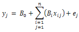 . From table 7, equation (23) for earth temperature at 5 cm below the earth surface is deduced as:
  | (23) |
From table 8, the equation (24) for the Earth temperature at 10cm below the ground surface is deduced for the earth temperature 10cm below the earth as:  | (24) |
Matlab programs for earth temperature at 5cm and 10cm were written to calculate the values of the computed earth temperature as shown in figures (2) to (13). The matlab programs are combination of matlab syntax on every line of statement. The data values for the environmental variables are imported into the matlab workspace, manipulated, stored into dummy variables, and assigned to environmental variables that appear in the regression equations, the programs are written and compiled on an m-file while the outputs are recorded on the matlab window. Figures (2) to (13) which show the tabulated data value for the observed and computed data round the year enables us to compare these values and our comparison shows that there is no significant difference between the computed and observed data values. Since the difference between the computed and observed values is insignificant, the computed data is used alternatively, instead of taking the measurement of ground temperature on a daily basis.Table 7. Coefficientsa Earth temperature 5cm
 |
| |
|
Table 8. Coefficientsa Earth temperature 10cm
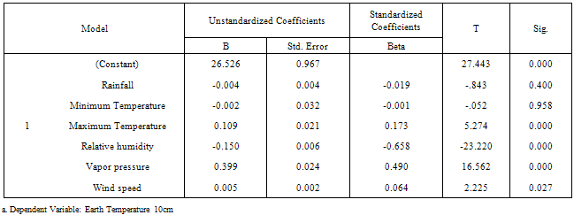 |
| |
|
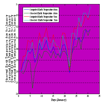 | Figure 2. Earth Temperature for January |
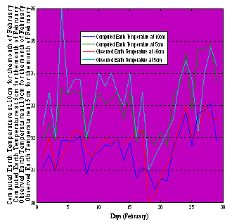 | Figure 3. Earth Temperature for February |
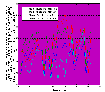 | Figure 4. Earth Temperature for March |
 | Figure 5. Earth Temperature for April |
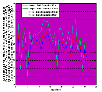 | Figure 6. Earth Temperature for May |
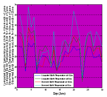 | Figure 7. Earth Temperature for June |
 | Figure 8. Earth Temperature for July |
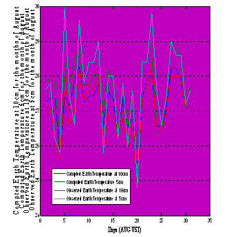 | Figure 9. Earth Temperature for August |
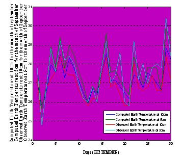 | Figure 10. Earth Temperature for September |
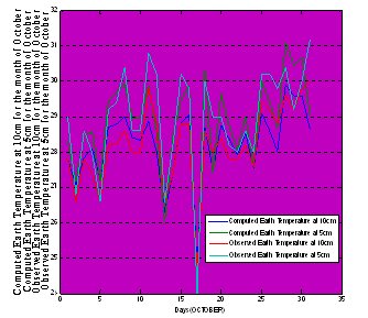 | Figure 11. Earth Temperature for October |
 | Figure 12. Earth Temperature for November |
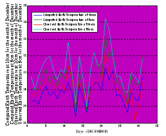 | Figure 13. Earth Temperature for December |
6. Conclusions
The models generated from the observed data as shown by equations (23) and (24) for the earth temperature at 5cm and 10 cm respectively by using Statistical Package for Social Science (SPSS) and assessed by matlab programming using the generated equations. The computed data were generated using the equations generated. Statistical test showed no significant difference between the observed data and the computed data, this prove that our computed data is effective as a substitute for the observed data within the assumed error limit.This work helps us to obtain the temperature of the ground at 5cm and 10cm below the ground, without going through the pain of measuring the earth temperature at these depths with a soil thermometer and without having physical contact with these quantities on the field on a daily routine. This work reduces expenses because you do not need to buy expensive temperature measuring element to predict the future temperature, we can generate the earth temperature of a location for as many years as possible, provided that data values for some of these environmental factors are available. This enables us to monitor fluctuation in ground temperature to avoid adverse effect on construction of roads, run ways, installation of underground cables and pipelines, depletion of nutrient under adverse temperature condition and growth and reproduction of plants.
Appendix : A matlab code for generating values for earth temperature at 5CM
%import the experimented data value for rainfall from the workspaceimport Rainfall.*i = 1:length(Rainfall);R= Rainfall;format long%import the experimented data value for the Minimum Temperature of the days from%the workspace import MinTempC.*j = 1:length(MinTempC);m0 = MinTempC;format short%import the experimented data value for the Maximum Temperature of the days%from the workspaceimport MaxTempC.*k = 1:length(MaxTempC);m1= MaxTempC;format short%import the experimented data value for the Relative Humidity of the days%from the workspaceimport Relhumidity.*l = 1:length(Relhumidity);H = Relhumidity;format short%import the experimented data value for the Vapour Pressure of the days from the workspaceimport vapPressure.*m = 1:length(VapPressure);v = VapPressure;format short%import the experimented data value for the WindSpeed of the days from the%workspaceimport Windspeed.*n = 1:length(Windspeed);W = Windspeed;format shorte0=((0.000*R)-(0.007*m0)+(0.026*m1)-(0.225*H)+(0.516*v)+(0.007*W)+(32.661))A matlab code for generating values for daily Earth Temperature at 10CM%import the experimented data value for rainfall from the workspaceimport Rainfall.*i = 1:length(Rainfall);R= Rainfall;format long%import the experimented data value for the Minimum Temperature of the days from%the workspace import MinTempC.*j = 1:length(MinTempC);m0 = MinTempC;format short%import the experimented data value for the Maximum Temperature of the days%from the workspaceimport MaxTempC.*k = 1:length(MaxTempC);m1= MaxTempC;format short%import the experimented data value for the Relative Humidity of the days%from the workspaceimport Relhumidity.*l = 1:length(Relhumidity);H = Relhumidity;format short%import the experimented data value for the Vapor Pressure of the days from the workspaceimport vapPressure.*m = 1:length(VapPressure);v = VapPressure;format short%import the experimented data value for the Windspeed of the days from the%workspaceimport Windspeed.*n = 1:length(Windspeed);W = Windspeed;format shorte0 =((-0.004*R)+(0.002*m0)+(0.109*m1)(0.150*H)+(0.399*v)+(0.005*W)+(26.526))
References
| [1] | Scheffran (2005) “Tools for stakeholder assessment and interaction”,http://www.esc.auckland.ac.nz/Organisations/ORSNZ/conf35/papers/BobCavana.pdf. |
| [2] | Scott Armstrong J. and Fred Collopy (1992). Error Measures For Generalizing About Forecasting Methods: Empirical Comparisons. International Journal of Forecasting 8: 69–80. |
| [3] | David H., (2005), “Introduction to Matlab for Engineering Students”, version 1.2, Northwestern University. |
| [4] | Mathworks (2011) “MATLAB programming Fundermentals” R2011b The Mathworks Inc. |
| [5] | Gunther G. and Weiss, (2007) “Introductions to Microcontrollers”, Vienna University of Technology, Institute of computer Engineering, version 1.4, |
| [6] | Pete Cockerell (Accessed 2012), ARM Assembly Language Programming. Available at:http://pete.cockerell.net/aalp/resources/pdf/all.pdf. |
| [7] | Olufolabi O.O. and Talabi C.O (2002) “Principles and Pratices of Statistics” first edition HAS-FAM (NIG.) enterprises |
| [8] | Linda E.L. (2003), “SPSS 12 Data Analysis Basics” Northern Illinious University Information technology service. |
 Abstract
 Reference
 Full-Text PDF
 Full-text HTML