-
Paper Information
- Next Paper
- Previous Paper
- Paper Submission
-
Journal Information
- About This Journal
- Editorial Board
- Current Issue
- Archive
- Author Guidelines
- Contact Us
International Journal of Theoretical and Mathematical Physics
p-ISSN: 2167-6844 e-ISSN: 2167-6852
2013; 3(1): 10-25
doi:10.5923/j.ijtmp.20130301.03
Lossless Transmission Lines Terminated by in-Series Connected RL-Loads Parallel to C-Load
 Abstract
 Reference
 Full-Text PDF
 Full-text HTML
Vasil G. Angelov
Department of Mathematics, University of Mining and Geology “St. I. Rilski”, Sofia, 1700, Bulgaria
Correspondence to: Vasil G. Angelov , Department of Mathematics, University of Mining and Geology “St. I. Rilski”, Sofia, 1700, Bulgaria.
| Email: |  |
Copyright © 2012 Scientific & Academic Publishing. All Rights Reserved.
The paper deals with an analysis of transmission line terminated by in series connected RL-loads parallel to C-load. The mixed problem for Telegrapher equations to a periodic problem on the boundary is reduced. The obtained neutral system of equations in an operator form is presented. The fixed points of the operator in question are solutions of the periodic problem.
Keywords: Lossless Transmission Lines, RLC-Loads, Periodic Solutions, Fixed Point Theorems
Cite this paper: Vasil G. Angelov , Lossless Transmission Lines Terminated by in-Series Connected RL-Loads Parallel to C-Load, International Journal of Theoretical and Mathematical Physics, Vol. 3 No. 1, 2013, pp. 10-25. doi: 10.5923/j.ijtmp.20130301.03.
Article Outline
1. Introduction
- The main purpose of the present paper is to consider a lossless transmission line loaded by in series connected nonlinear RL-loads parallel to C-load. Such a configuration arises not only in radio frequencies devices but in various geophysical studies as well (cf.[1]). Our goal is to demonstrate the advantages of our method[2] used in analogous problems. So we came up with an approach to solve this set of problems (cf.[3]-[7]).The primary purpose of the present paper is twofold. First, to formulate the mixed problem for hyperbolic Telegrapher equations corresponding to the nonlinear circuits on Figure 1. The boundary conditions are nonlinear ones in view of the nonlinear characteristics of the loads. Important first step on the base of Kirchoff’s law is to derive the boundary conditions in the form of differential equations on the boundary. This is done in 2.1. Reducing the mixed problem to a neutral system on the boundary is made in 2.2 following the technique from[2],[5] and[6]. Second, to present a method for solving neutral equations with “bad” (non-Lipschitz) nonlinearities. In 2.3 the domains of the nonlinear characteristics are defined. They have to possess strictly positive lower bounds and namely Assumption (C) for capacitive functions and (L) for inductive functions ensure that. In 2.3 the choice of functional spaces and a family of pseudo-metrics is directly related to the operator representation of the periodic problem in 2.4. Let us point out that the extension of Bielecki norm allows to overcome the difficulties caused by nonlinearity of the characteristic functions. The key role plays Lemma 3. It guaranties that the fixed points of the operator defined in 2.4 are periodic solutions of the neutral system and conversely. The main result is Theorem 1 (cf. 2.5) and its proof consists of two parts. The first one is to show that operator B maps the set
 into itself. The second one is to show that B is contractive operator. The fixed point of B is the required periodic solution. The numerical example in 2.6 shows that for applications are required only inequalities obtained in the proof of the main theorem.
 2. Main Results
2.1. Formulation of the Problem
- Let
 be the length of the transmission line and
  , where L is per unit length inductance and C – per unit-length capacitance. In accordance of Kirchoff’s voltage-law (Figure 1) we have to add the voltages of the elements
  and
and  after that to define the current of
  and finally to add it with the current of
  . In the real cases parallel to
  and
and  is connected an input voltage
  , where
  is the amplification coefficient. Since we have to add the currents one can replaced
  by an equivalent current source
  . We assume that the second end is terminated by the same configuration.Assume that
  and
and  are nonlinear elements, that is,
  and
and  are nonlinear functions. So we have
 and then
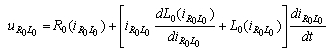
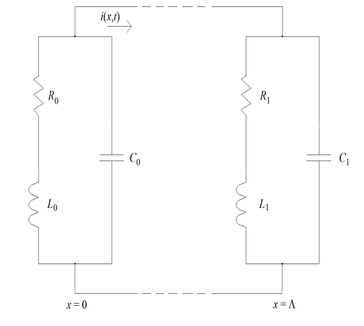 | Figure 1. Lossless transmission line terminated at both ends by in series connected RL-loads parallel to C-load |
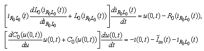
 is connected parallel to RL-elements then Kirchoff’s current-law yields
  | (1) |
 then
then  can be found as a solution of differential equation
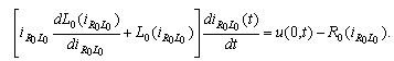 But
But  is unknown too and then from (1) we have
 or one more differential equation:
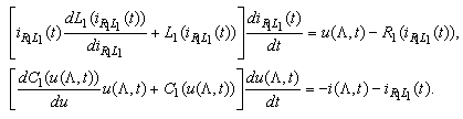
 Analogously for the right end we have
 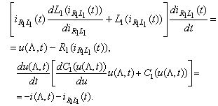 Now we are able to formulate the initial-boundary value (mixed) problem for the transmission line equations: to find a solution
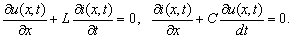
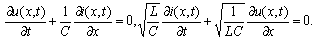
  of the first order partial differential system of hyperbolic type
 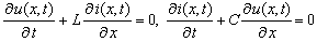 | (2) |
 satisfying the initial conditions
 | (3) |

 | (4) |

 | (5) |
2.2. Reducing the Mixed Problem to an Initial Value Problem on the Boundary
- We proceed from the lossless transmission line equations
 | (6) |
 | (7) |
 we get:
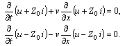 | (8) |
 and hence
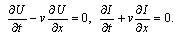 It follows
 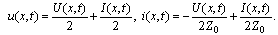 | (9) |
 and
and  we have
 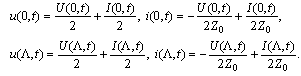 Replace them in (4) and (5) we obtain
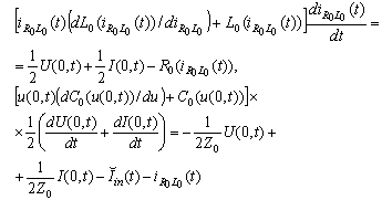 and
and 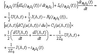 But
But We assume that the unknown functions are
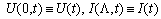 and then in view of
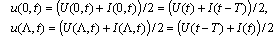 solve with respect to the derivatives we reach the system
 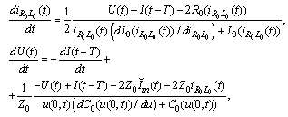 | (10) |
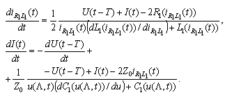 So we have obtained a neutral system of differential equations with retarded arguments.
2.3. Estimates of the Arising Nonlinearities and Introducing Metrics
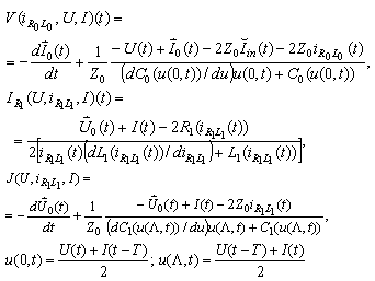
- We consider C-V characteristics
 , for
, for where
where  have a strictly positive lower bounds. Put
  ..Then
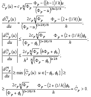 For the I-V characteristics we assume
 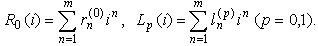 Then
Then  . For
. For  we get
 Assumptions (L):
 Assumptions (C):
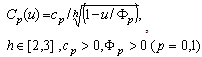
 For the V-I characteristics we assume that they are of polynomial type:
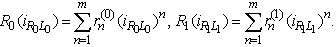 We introduce the sets for the unknown functions
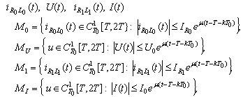

 where
where  is the set of all continuously differentiable
  -periodic functions and
  are positive constants (chosen below) and
  Introduce the metrics
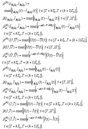 The set
  turns out into a complete metric space with respect to the metric:
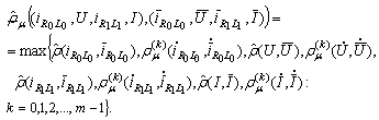
2.4. Operator Presentation of the Periodic Problem
- Now we formulate the main problem: to find a
 -periodic solution
  of the system (10) on the interval
  coinciding with prescribed
  -periodic initial functions
 on the interval respectively:
 Remark 1. As in[3] one can shift the initial function of the mixed problem from the interval
  along the characteristic to the interval
  The main difficulty is to define a suitable operator whose fixed points are solutions sought. We define it in the following way: the four-tuple functions
  are defined on every interval
  (for every k = 0,1,2, …, m-1) by the expressions
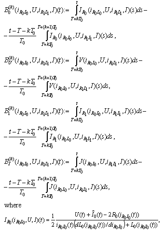
 and
and  are translated to the right initial functions
  over
over  .From now on the following assumptions will be fulfilled:(E):
 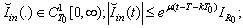 (IN):
(IN): 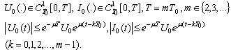 It follows
  Lemma 1. If (E) and (IN) are satisfied and
  then
then 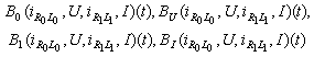 are
are  -periodic ones.Lemma 2. If
  then
then
 The proofs can be accomplished as in[5],[6].The following lemma guaranties that the fixed points of the above defined operator are periodic solutions of the neutral system (10).Lemma 3. The periodic problem (10) has a solution
 that is,
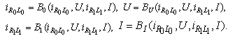 Proof: Let
 be a
be a  -periodic solution of (10). Then after integration of the first equation we have (recall that
  ):
): 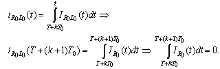 Therefore
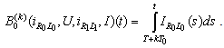 Analogously we obtain
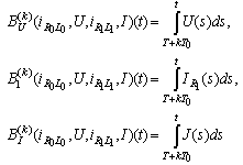 that is,
 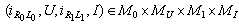 is a fixed point of B.Conversely, let
  have a fixed point
  Then
Then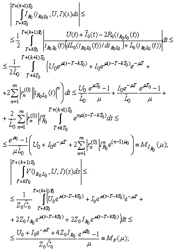
 If we assume
 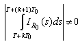 in view of
  one obtains a contradiction. It follows
 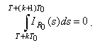 Analogously
 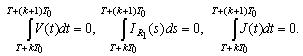 Consequently
 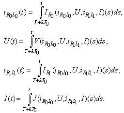 Differentiating the last equalities we conclude that (10) has
  -periodic solution.Lemma 3 is thus proved.
 2.5. Existence-Uniqueness of Periodic Solution
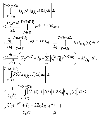
- The main result contains in the followingTheorem 1. Let assumptions (L), (C), (E) and (IN) be fulfilled. Then there exists a unique T0-periodic solution of (10).Proof: We show that
 maps
maps  into itself. Indeed
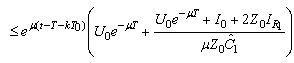
 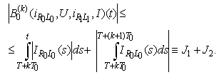 We have
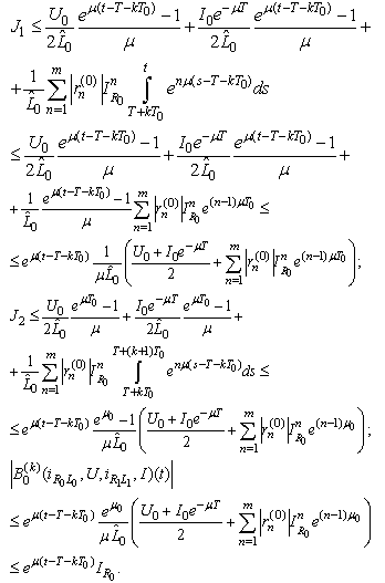 Further on we have
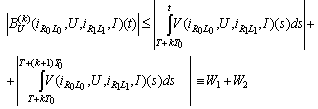 and
and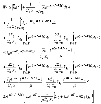 and
and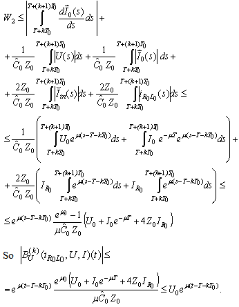 On the other hand
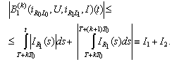 We have
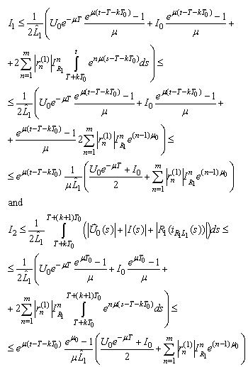 Then
Then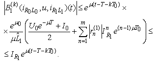 Finally
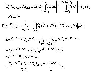
 and
and It remains to obtain the Lipschitz estimates for the right-hand sides of the equations. Omitting calculation of the partial derivatives we obtain:
 Then
Then
 It follows
 Further on we get
 It follows
 For the third component we obtain:
 For the fourth component we have
 It follows
 For the derivatives we obtain
 Consequently
 Further on we have
 ThereforeConsequently
 Further on we have
  Then
Then For the last component of the derivative we obtain
 and
and On the other hand
 Consequently
 .Finally we have
  where
where  Then B has a unique fixed point which is a periodic solution of (10).Theorem 1 is thus proved.
 2.6. Numerical Example
- For a transmission line with length


 Then
Then  .Let us check the propagation of waves with
  . We have
 We choose
  , then
  and
and .We choose resistive elements with the following V-I characteristics
 and inductive elements with
  Then
Then  For
For  one obtains
 .Let us take
 where
where  . Let us choose
 and
and
 . Then

 .Then the above inequalities for


 become:


 We calculate just
  since
since  are of order
  :
:  ;
;  ;
;  ;
;  .
.3. Conclusions
- We consider transmission lines neglecting the lossies. This makes it possible to find conditions for the existence and uniqueness of periodic regimes. This natural physical fact is confirmed by the mathematical method we apply. • In order to prove an existence-uniqueness theorem we introduce an operator (unknown in the literature up to now) whose fixed points are periodic solutions of the problem stated. We apply contractive fixed point theorems in metric spaces. By extended Bielecki metrics we overcome the difficulties caused by polynomial and transcendental nonlinearities.• The numerical example demonstrates a frame of applicability of the theory exposed (for instance to design of circuits) and shows that the method could be applied checking few simple inequalities between the basic specific parameter of the lines and loads.• We show a unified approach for solving problems for analysis of transmission lines terminated various configurations of nonlinear loads. In contrast to various results devoted to numerical methods[8]-[14] we obtain an explicit approximated solution. • We emphasize on the fact that first we prove not only an existence but and uniqueness of the solution as well. So our successive approximations tend to this solution. All other methods need such a uniqueness result. Unfortunately in most papers the uniqueness is not ensured.