1. Introduction

The motion of continuous media is often accompanied by the formation of transitional zones of strong gradients, where flow parameters (velocity, density, pressure, temperature, etc.) vary rapidly. If dissipative mechanisms are neglected, then such thin zones are usually treated as surfaces of strong discontinuity. In that case the flow parameters change step-wise with jumps on a propagating surface of strong discontinuity (e.g., shock wave). Note that motions of ideal continuous media are usually described by hyperbolic conservation laws for which the mathematical theory of shock waves has been well discovered not only for one-dimensional[1–10] but also for multi-dimensional flows[11–21].

Concerning continuous media with dissipation (e.g., viscosity, heat conduction, etc.), transitional zones of strong gradients can also be formed, and there emerges the necessity for the mathematical modeling of such a phenomenon. In this paper, we are concerned with the motion of a viscous compressible gas in the framework of the Navier-Stokes model. As is known, the Navier-Stokes equations are applied for solving the problem on shock structure in a viscous and heat conducting gas (see, e.g., the classical approach in[22]). In this problem, instead of a surface of strong discontinuity one considers a thin transitional zone (viscous profile) where flow parameters vary continuously.

A strong discontinuity in an ideal medium is said to have a viscous profile (or structure) if the discontinuous flow is a limiting one under vanishing dissipation[22–25]. Although, it should be noted that until now such a viscous profile (continuous) approach was applying for different concrete models of continuum mechanics mainly in the one-dimensional case. So, it cannot be fully considered as an alternative one to the discontinuous approach for multi-dimensional shock fronts. At the same time, for continuous media with dissipation only the continuous approach has yet a sufficient justification (at least, on the one-dimensional level[26]).

The indirect confirmation of the correctness of precisely this continuous approach for viscous conservation laws is the following. Hyperbolic conservation laws modeling motions of ideal media have such a property that their solutions are continuous and single-valued during short time only (even for rather smooth initial data). After that the so-called gradient catastrophe occurs (see, e.g.,[10]), and one has to introduce strong discontinuities. Solutions of viscous conservation laws have apparently no such a property. This is indirectly confirmed by numerous results (e.g.,[27–30]) concerning global existence theorems for the Navier-Stokes equations.

In this connection, we especially refer to interesting results in[30] where the global existence and uniqueness of the weak solution of the one-dimensional Navier-Stokes equations written in the Lagrangian coordinates has been proved for the case of discontinuous initial data. Under certain natural restrictions on the initial data it was shown that shock discontinuities do not arise in solutions of the Navier-Stokes equations.

At the same time, it should be noted that in some works (their number is not small) the discontinuous approach is nevertheless used for shock waves in a viscous gas. For example, to estimate the influence of a small viscosity to the evolution of perturbations of planar gas dynamic shock waves it is assumed in[31] that one can neglect the width of the shock layer. Therefore, as for an inviscid gas, the problem on the evolution of perturbations is reduced in[31] to the study of a linear initial boundary value problem with boundary conditions on a shock front obtained by the linearization of the generalized Rankine-Hugoniot relations. Another example is the numerical analysis of two-dimensional steady viscous flows near blunt bodies[32] (we just refer to[32] as to a typical paper from numerous computational works relating to the subject under discussion). To bound essentially the calculated domain, where solutions of the compressible Navier-Stokes equations are sought, one introduces a bow shock that is treated in[32] as a strong discontinuity on which surface the generalized Rankine-Hugoniot conditions hold. Moreover, steady flows were being computed in[32] by the stabilization method, i.e., steady-state solutions of the Navier-Stokes equations were being sought as a limit of unsteady ones under .

In[33–35], on the example of the compressible Navier-Stokes equations the groundlessness of the approach based on the consideration of shock waves in a viscous gas as fictitious surfaces of strong discontinuity was shown. It appears that this conclusion can be already drawn according to the linear analysis. For this purpose one studies the initial boundary value problem (IBVP) obtained by the linearization of the Navier-Stokes equations and the jump conditions with respect to their piecewise constant solution. This piecewise constant solution describes the following flow regime for a viscous gas: a supersonic steady viscous flow (for) is separated from a subsonic one (for) by a planar shock discontinuity (with the equation). It was shown in[33–35] that this planar shock wave is unstable depending not on the character of linearized boundary conditions at. This is a direct consequence of the fact that the number of independent parameters determining an arbitrary perturbation of the shock front is greater than that of the linearized boundary conditions. That is, the shock wave in a viscous gas viewed as a surface of strong discontinuity is like nonevolutionary (undercompressive) discontinuities in ideal media (see[36,37]).

Mathematically, the exponentially increasing particular solutions constructed in[33–35] for establishing linear instability are, actually, Hadamard-type examples (see, e.g.,[14,38]) that indicate the ill-posedness of the linearized stability IBVP mentioned above. The discovered instability can be also treated as an indirect proof of the inadmissibility of steady-state calculations for viscous blunt body flows with a bow shock discontinuity. From the physical point of view, this means the practical unrealizability of the steady flow regime for a viscous gas described above.

At the same time, accounting for some advantages of the discontinuous approach (especially for numerical calculations), one would like to modify this approach so that it might be applied (together with the stabilization method) with a mathematical ground for steady-state calculations for blunt body flows with dissipation. In[39,40], on the example of the linearized stability problem for the shock discontinuity in a viscous gas the idea of such a modification was proposed for the one-dimensional case. The essence of this idea is that for the original shock front problem one writes additional boundary conditions so that for the modified problem the steady flow regime with a shock wave described above becomes asymptotically stable (by Lyapunov). That is, at least on the linearized level this might justify the stabilization method which can now be applied for finding (e.g., numerically) steady flow regimes for a viscous gas with a shock wave. The mentioned additional boundary conditions were suggested to be written with regard to an a priori information about steady-state solutions of the Navier-Stokes equations being sought by the stabilization method.

In the present paper we consider a curvilinear shock wave.

2. Preliminary Information

2.1. The System Describing Gas Dynamics

Recall that in[33,39] the stability of shock waves in a compressible viscous gas described by the well-known Navier-Stokes equations was studied. Let us consider the same flow regime as in[33,39] (see Fig. 1): the supersonic steady viscous flow is separated from the disturbed flow by a shock wave with the equation

(1)

where is the time, is the Cartesian coordinate system (in this paper we restrict ourselves to the consideration of the planar case).

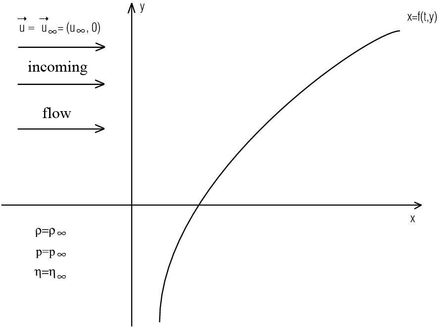Figure 1. Viscous gas flow with a shock wave

We write down the Navier-Stokes equations for a compressible heat-conducting polytropic gas in the Cartesian coordinate system in dimensionless form as (see[33,39,41])

(2)

Here is the gas density, is the specific volume, are the Cartesian components of the velocity vector, is the pressure,

are constants,

, are the first and second viscosity coefficients (see[39,41]),

is the Reynolds number (see[41]),

is the temperature, is the Prandtl number (see[41]),

is the heat conductivity,

;, are the specific heat capacities,

the following scaling factors were used to define the dimensionless time, the coordinates, , the density, the velocity components, , the pressure (see Fig. 1): , , , , , where is a characteristic length (see also Remark 2.1); the dimensionless viscosity coefficients, are defined by using as the scaling factor; the viscosity coefficient depends on according to the power law (see[41])

(3)

where is the Mach number for the upstream flow, is a constant.

2.2. Rankine-Hugoniot Conditions

On the surface of shock wave (1) generalized Rankine-Hugoniot conditions hold (see[33,39]). Using some cumbersome manipulations they can be reduced to the following

(4)

(5)

(6)

(7)

Here

2.3. The Problem Written in the Curvilinear Coordinate System

Further we will need the Navier-Stokes equations (2) rewritten in orthogonal curvilinear coordinates:

(8)

and in (8) are the dimensionless coordinates. Formulae (8) can be rewritten in the dimensional form as

(8a)

where is a characteristic length (see Remark 2.1). The curvilinear coordinates, are chosen so that the front of the shock wave is described in the stationary case by the equation (see Fig. 2)

(1a)

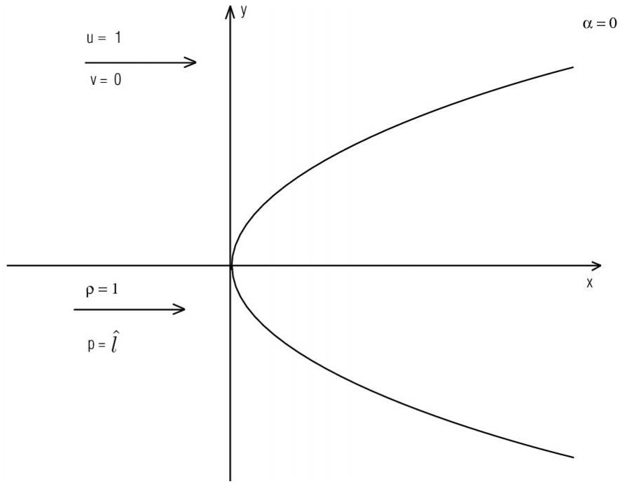Figure 2. Front of the shock wave

Remark 2.1. Note that the radius of curvature of the stationary shock wave at can be taken as the characteristic length

We rewrite the Navier-Stokes equations in the coordinates in the following nonconservative form (see[41]):

(9)

(10)

(11)

(12)

where

, are the physical components of the velocity vector in the curvilinear coordinates related to the Cartesian components, as

(13)

where, are the so-called contravariant components of the velocity vector (see[42]);

(14)

(15)

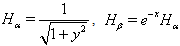are the Lamé coefficients (see[42]),

Remark 2.2. Taking into account formulae (13), we can rewrite equations (9)–(12) as

(9a)

(10a)

(11a)

(12a)

Here

the values of, are calculated by using (14), (15).

Remark 2.3. We are also interested in stationary solutions to equations (9)–(12) (or (9a)–(12a)) with boundary conditions set at the front of the shock wave (see Fig. 2). In the stationary case conditions (4)–(7) take the following form:

(4a)

(5a)

(6a)

(7a)

where.

3. Solving the Stationary Navier-Stokes Equations in a Neighborhood of the Line

3.1. Additional Assumptions

The system of equations (9a)–(12a) is too complicated. Let us modify it in a certain way in the stationary case. To simplify further calculations we will assume that

a) the viscosity coefficient (see formula (3)) is constant behind the shock wave:

(3a)

where, are constants;

b) , i.e., the Prandtl number;

c) , where is a new dependent variable;

d) the functions, are denoted as,.

Then in the region the system (9a)–(12a) in the stationary case can be rewritten as

(16)

(17)

(18)

(19)

where,

For the solution of system (16)–(19) should satisfy relations (4a)–(7a) which under assumptions a) – d) cited above can be rewritten as follows:

(20)

(21)

(22)

(23)

Here

In addition, we will assume that the functions , satisfy the so-called ''soft condition'' (see[41]) as:

(24)

3.2. The Taylor Expansion with Respect to the Argument β

Further we will simplify the nonstationary system (9a)–(12a) using stationary solutions , in a neighborhood of the line for definition of system’s coefficients. The functions, , , are even with respect to the argument (see Fig. 2). Therefore, in a neighborhood of the line we will search them in the form of the following series (see[43,44]):

(25)

Remark 3.1. Using formulae (8), we can also expand the functions, into series with respect to the variable.

Substituting expansion (25) into (16)–(24) and equating the coefficients at the same powers of beta , we obtain a relation for determining the functions, , , , etc. in series (25). Equating the coefficients at, we have:

(26)

(27)

(28)

(29)

for;

(30)

(31)

(32)

(33)

for;

(34)

Here

ect.

Remark 3.2. As follows from (26)–(34), for the determination of the functions, , , we have to know the functions , ,. Further, assuming in these relations that, , , we will consider an approximate solution of the problem (26)–(34).

Remark 3.3. We set in formula (3a) that,. From (33), (31) we have:

(35)

Let also in formulae (3), (3a). Then, it follows from (30), (31), (35) that

(36)

where.

3.3. The Boundary-Value Problem of Second Order for the Components of Velocity Vector

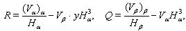
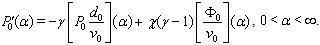
Let us return to the boundary-value problem (26)–(34). From (26), (27) we have:

(37)

Here

and the quantity can be expressed in terms of by formula (36). Let us rewrite equations (28), (29) as follows:

(38)

(39)

where,

The boundary conditions for equations (38), (39) follow from (36), (32), (34):

(40)

(41)

(42)

For searching approximate solutions of the boundary-value problem (38)–(42) a new computational algorithm was proposed. It is described in the section 5, where we also present results of numerical experiments.

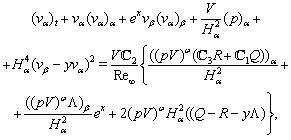
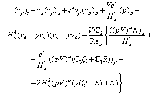
4. The Linearization of Nonstationary Problem for System (9a)–(12a)

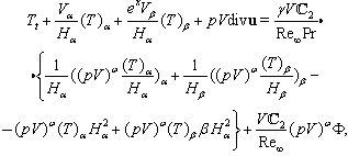
4.1. The Linarization of Nonstationary Equations (9a)–(12a)

Let us linearize of system (9a)–(12a) about the basic solution (25) and freeze then the coefficients of the linearized system on the line. Denoting small perturbations by the same letters, we finally obtain:

(43)

(44)

(45)

(46)

Here

System (43)–(46) is considered in the domain (at infinity the sought functions tends to zero).

Let us simplify system (43)–(46) by freezing the functions and at the point and making the change of (below we drop tilde and again write instead of). We get finally that

(43a)

(45a)

(46a)

Where

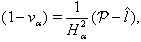
4.2. The Linearization of Stationary Boundary Conditions (4a)–(7a)

Let us now formulate boundary conditions at. To this end we linearize conditions (4a)–(7a) posed at, where the function is the small perturbation of the shock front which unperturbed position is. Freezing the coefficients at we will finally obtain:

(47)

(48)

(49)

(50)

Here

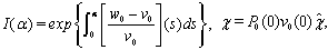
Remark 4.1. According to [33,39] for the determination of the function describing the small perturbation of the shock front we will add to (43a)–(46a), (47)–(50) the equation in the form (see, for example,[33,39])

where is a constant.

where .

Remark 4.3. We also assume that the small perturbations

(see (24)).

In the section 5 a new computational algorithm for finding stationary approximate solutions of the initial-boundary value problem (43a)–(46a), (47)–(51) is described, where we also present results of numerical experiments.

5. A New Computational Algorithm for Solving Boundary-Value Problems of Second Order

Now we will propose a new numerical algorithm for solving the problem (38)–(42). In numerical calculations we pass from infinite segment to a finite one and assume that, where is a large enough number. We make the change of variable. Let (do not forget that ) , then . Note also that has no physical meaning and dimension and the new notation is not equal to that from section 2 and concerns only sections 5 and 6.

5.1. The Nonstationary Regularization and the Stabilization Method

Introducing the notations

, we rewrite the boundary-value problem (38)–(42) as follows:

(52)

with the boundary conditions

(53)

at and

(54)

at. Here

For searching approximate solutions of the boundary-value problem (52)–(54) we will use the stabilization method. To this end let us apply to the equations of system (52) the nonstationary regularization proposed in the[45,46]. As a result, we obtain the system of nonstationary equations

(55)

(56)

Here and t plays the role of time, i.e., we assume further that the unknowns, depend also on the variable t:.

Remark 5.1. The main idea of the stabilization method is described, for example, in[47]. In our case for the implementation of the stabilization method we should discretize the nonstationary equations (55), (56) by time and perform numerical computations until the solution ''stabilized''. In other words, the algorithm using this method will stop only when the norm of the difference of the solutions at next and previous time layers becomes small enough. Thus, we search a solution of problem (52)–(54) in the form of a limit as of the solutions of the nonstationary equations (55), (56) with the boundary conditions (53), (54).

For the application of the stabilization method it is necessary to specify initial data for system (55), (56). Further we assume that

(57)

Using the idea of the method of lines (see[45,46]), we discretize with respect to t equations (55), (56). To this end we introduce the notations

where is the time-step of the greed.

Approximating the derivatives , in (55), (56) by the expressions and respectively, we obtain

(58)

(59)

where

5.2. The Spline-Function Technique

We will seek a solution of equations (58), (59) in the form of cubic interpolation splines (see[45,46,48]). For example, let us write the approximate solution of equation (58) in the following way:

(60)

where

The cubic spline (60) should be continuous together with its first derivative on the whole segment (the second derivative is continuous according to the definition of spline (60)).

The first derivative of the cubic spline has the following form:

Then, computing the aggregates

where

and equating them, one gets

(61)

Here

Assuming in (58) and substituting from (58) into (61), one gets the following three-pointed difference scheme:

(62)

where

The derivatives at the grid nodes (i.e., at the points ) are required for computing the right-hand sides and on the next time layer. These derivatives can be computed using spline (60).

Since where , then

Using similar arguments, we get the three-pointed difference scheme

(63)

for finding a solution of equation (59), where The derivatives can be found as follows:

Replacing in (53), (54) the derivatives , , by their difference analogues ,

we obtain the boundary conditions on the th time layer

(64)

for scheme (62) as well as the boundary conditions the on th layer

(65)

for scheme (63). Here

5.3. The Use of Sweep Method

Equations (62), (63) with the boundary conditions (64), (65) can be solved by using the sweep method. Let us describe the application of this method on the example of problem (62), (64). The computations for scheme (63) with the boundary conditions (65) can be done in the same manner.

We write down system (62) in the form

(66)

The boundary conditions (64) are rewritten as follows:

(67)

(68)

Where

Remark 5.2. Problem (63), (65) can be also easily reduced to the problem of form (66)–(68).

According to the idea of the sweep method we search a solution of (66)–(68) as

(69)

Substituting (69) into (66), we find recurrent formulae for the sweep coefficients :

(70)

For we take the values of the sweep coefficients from the boundary condition (67). Thus, in the cycle of the forward sweep we can find the coefficients by formulas (70). Then, using the boundary condition (68) and formula (69), we can compute the solution at the point :

At last, knowing and the coefficients of the sweep method, we can find a solution of problem (62), (64) by formula (69) in the cycle of the backward sweep.

Remark 5.3. Using the same arguments, we can find a solution of problem (63), (65) by applying again the sweep method (see Remark 5.2).

5.4. The Computational Scheme and Numerical Results

As a result, the scheme of searching approximate solutions of system (55), (56) at each time layer is the following. Starting from the values of unknowns obtained on the th time layer we compute the values of variables of the problem and the right-hand side at each point of the space greed. Then we find the solution of equation (55) with boundary conditions (53), (54) by using the sweep method. After that we compute the values of variables and right-hand side by taking into account the obtained and solve the boundary-value problem (56), (53), (54). At last, we get the solution of system (55), (56) at the th time layer. Then, we pass to the next time layer.

According to the idea of the stabilization method (see Remark 5.1), these actions should be repeated until the solution becomes ''stabilized''. The obtained values of unknowns are exactly the desired approximate solution of the boundary-value problem (52)–(54).

For the organization of computations by the proposed scheme it is necessary to specify the list of physical and numerical parameters. In Table 1 we give the description of each parameter and the range of its values.

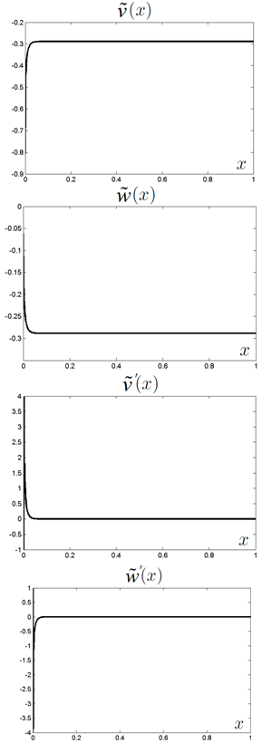Figure 3. The functions and and their derivatives obtained after computations with the parameters , , , , , , ,

Table 1. Physical and Numerical Parameters

Another important parameter is the relative computational accuracy . The algorithm stops if

Some results of computations are given in Fig. 3.

6. Numerical Results Showing the Stability of Shock Wave

6.1. The Fourier Transform for Nonstationary Problem (43a)–(46a), (47)–(51)

Now let us describe the algorithm of searching approximate stationary solutions of equations (43a)–(46a) for small perturbations with the boundary condition (47)–(51). As it was made in the section 5 the stationary solution will be find with a help of the stabilization method. Following section 5, we assume that , where is large enough, replace the variable by and denote , (do not forget that ). Then

Assume that at the unknowns of problem (43a)–(46a) satisfy initial data (see Remark 4.2).

Remark 6.1. In the section 4 the computational algorithm for searching the values of functions and was described in detail. In this case the functions and needed for the determination of the coefficients of equations (43a)–(46a) can be expressed as follows:

Let be the Fourier transform of the velocity component with respect to the variable , where is the Fourier parameter (the notation corresponds only to this section, in other sections is a constant from (3))::

(71)

It is known that the Fourier transform of the derivatives has the form

Similarly we can find the Fourier transforms of the unknowns, , and their derivatives. Applying then the Fourier transform in form (71) to each equation in (43a)–(46a) and each condition in (47)–(51) and dropping the hats, we get the system

(72)

with the conditions

(73)

on the boundary and

(74)

on the boundary.

Assuming and to be complex-valued functions in the form

we substitute them into (72)–(74) and equate the corresponding real and imaginary parts in the obtained relations. Finally we derive

(75)

(76)

(77)

(78)

Here

The boundary conditions for (75)–(78) at obtained from (73) have the form

(79)

(80)

(81)

(82)

Using (74), we find the boundary conditions

(83)

(84)

For (75), (76) at.

6.2. The Numerical Solution of Boundary-Value Problems

Let the function be one of the unknowns , , and the function be the corresponding right-hand side, , or. Then, the equations (75), (76) can be written in the general form

(85)

Each of the boundary conditions (79), (80) can be represented as

(86)

and the conditions (83), (84) are

(87)

Remark 6.2. The coefficients, , can be written after elementary arithmetical transformations of equations (75), (76) and the boundary conditions (79), (80).

Let the function be one of the unknowns, , , and the function be the corresponding right-hand side, , or. Then, equations (77), (78) can be written in the general form

(88)

Each of the boundary conditions (81), (82) can be written as follows

(89)

Remark 6.3. The coefficient takes the values, , or (see (81), (82)).

Our goal is finding approximate solutions of problem (75)–(84) with certain initial data. To this end we use the idea of the method of lines and discretize the nonstationary equations (85), (88) with respect to the variable tIntroduce the notations

where is the step of the time greed.

Approximating the derivatives,

in (85), (88) by expressions and respectively, one obtains

(90)

where, ,

(91)

Let us discretize the relations (90), (91), (86), (87), (89) with respect to the variable x. We introduce on the segment a uniform grid with the nodes, and the step, where is the number of greed nodes. Let, , and be the values of the unknowns, , , at the th greed node. Considering the boundary conditions (86), (87) on the n time layer and replacing there the derivative on the boundaries and by its difference analogues and, one obtains the following boundary-value problem for equation (90):

(92)

Remark 6.4. In section 5 we described an effective computational algorithm for searching solutions of boundary-value problems in form (92) and based on the spline functions technique and the sweep method.

Replacing in equation (91) the derivative at the point by its difference analogue, and taking into account (89), one gets

or

(93)

Here is the value of at the point . Thus, knowing the quantities and from the previous time layer at each point and from the current layer and using (93), we can find at the current time layer.

6.3. The Computational Scheme and the Results Obtained

Thus, at each time layer we can find the values of the unknowns of problem (75)–(84) as solutions of the boundary-value problems (92), (93). Then, using these values, we recompute the right-hand sides , of equations (75)–(78) and pass to the next time layer (on the first layer the values of the right-hand sides can be found from the initial data). Choosing n large enough, we can finally find the approximate stationary solution of problem (75)–(84) and, hence, the approximate stationary solution of the original problem (43a)–(46a), (47)–(51) for large enough values of time.

Figure 4. The functions, and obtained in the computations with the parameters, , , (see Table I)

The results of the numerical computations obtained with the help of the described algorithm are given in Fig. 4, where one can see the stationary solutions for small perturbations and . These graphs show that the obtained values are sufficiently close to zero. This fact is the evidence of the stability of the shock wave in a compressible viscous gas with given parameters.

ACKNOWLEDGEMENTS

The authors are indebted to prof. Yu.L.Trakhinin for the help in the preparation of the manuscript of this paper, to prof. D. L. Tkachev and Ph. D. R. S. Bushmanov.