Minoru Fujimoto 1, Kunihiko Uehara 2
1Seika Science Research Laboratory, Seika-cho, Kyoto, 619-0237, Japan
2Department of Physics, Tezukayama University, Nara, 631-8501, Japan
Copyright © 2012 Scientific & Academic Publishing. All Rights Reserved.
Abstract
We have proposed a regularization technique and applied it to the Euler product of the zeta functions in the part one. In this paper that is the second part of the trilogy, we aim the nature of the non-trivial zero for the Riemann zeta function which gives us another evidence to demonstrate the Riemann hypotheses by way of the approximate functional equation.Some other results on the critical line are presented using the relations between the Euler product and the deformed summation representations in the critical strip. We also discuss a set of equations which yields the primes and the zeros of the zeta functions. In part three, we will focus on physical applications using these outcomes.
Keywords:
ZetaFunction, Riemann Hypothesis, Prime Numbers, Non-Trivial Zeros
1. Introduction
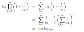
In the situation that the regularizations by the zeta functionhave been successful with some physical applications,[2][5][13,14] we proposed a regularization technique[7] applicable to the Euler product representation and gave an evidence for the Riemann hypotheses by using this technique in the part one. In this part, we now focus on the zeros of the Riemann zeta function and the surrounding properties of the zeros including other evidences to demonstrate the Riemann hypotheses.[1] The Euler product representation, which played an essential rolein the first part, will be interpreted in terms of the summation representation on the critical line .The definition of the Riemann zeta function is
 | (1) |
for , where the right hand side is the Euler product representation and pk is the k-th prime number. Hereafter we adopt a notation
  such as
 | (2) |
which is well regularized even in the critical strip . Considering the approximate expansion formula for the Riemann zeta function, we propose an evidence for an elegant proof of the Riemann hypothesis in section 2.and in§3we show surrounding properties of the zeros for the Riemann zeta function by deforming the Euler product representation to the summation form on the critical line. We study the relation between the primes and the zeros of the zeta function in connection with the Sato-Tate conjecture in section 4, and we will discuss the equations for these primes and zeros in§5.
2. The Expansion Formula and the Riemann Hypothesis
The Euler-Maclaurin sum formula is given by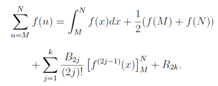 | (3) |
whereB2j is the 2j-th Bernoulli number and the remainder term: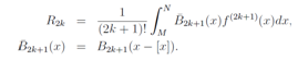 | (4) |
We parametrize a complex variable z by two real variable such as z = s(1/2+ it) as sameas that in the first part. Using the Euler-Maclaurin sum formula on the assumption of , we get the relation
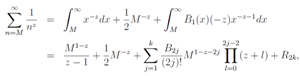 | (5) |
where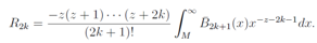 | (6) |
As is well known we can go forward to the expansion formula in the case of ,
, | (7) |
The remainder term R2k can be estimated as follows: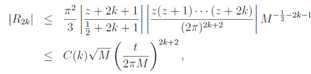 | (8) |
where we put s = 1 and C(k) is constant only depending on k. This tells us that it is necessary for the remainder term to be  to converge. Taking account of the Euler-Maclaurin sum formula, we can put the regularized zeta function as
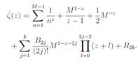
 | (9) |
and a zero in the critical strip is the solution to the equation | (10) |
These equations (9) and (10) are identical to the equation (A4) in the first part. As stated in Appendix A in the first part, Eq.(2) can be derived by way of the regularization method developed in the part one, which means that we can reach here besides using the Euler-Maclaurin sum formula. As (1 −ρ) is also the solution when ρ is the solution of Eq.(10), asolution of the equation | (11) |
is also a zero. Now we transform Eq.(9) to | (12) |
and substituting (1−z) for z, we get | (13) |
Combining these equations (12) and (13), we get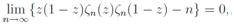 | (14) |
namely,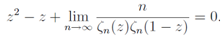 | (15) |
The solution ρn of the equation  is satisfied the relation
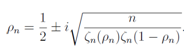 | (16) |
On the other hand, the approximate functional equation by Hardy and Littlewood[4], which leads to the Riemann-Siegel formula, is given by 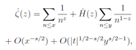 | (17) |
where is given by
 | (18) |
For s>2, the relation | (19) |
is satisfied and we write down  as,
as, | (20) |
Then the relation | (21) |
is satisfied for  and substituting (1−z) for z, we conclude Eq.(21) is satisfied for all z.We set
 , then
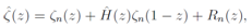 | (22) |
where the remainder term Rn(z):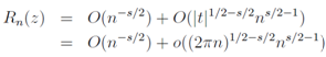 | (23) |
can be ignored by taking the limit of n→∞, namely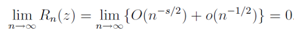 | (24) |
We put the relations at zeros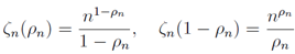 | (25) |
into Eq.(22) together with  , we can write
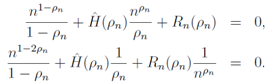 | (26) |
Taking the limit of n →∞, we get the relations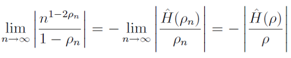 | (27) |
he right hand side of Eq.(27) is finite, so the numerator of the left hand side  must be finite. This means that the real part of (1 −2ρn) must converge to 0 in the limit of n →∞when the real part of (1 −2ρn) is positive. When
  , we rewrite the left hand side of Eq.(27) like
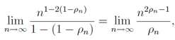 | (28) |
so we get the same goal as  . After all, the Riemann hypothesis is satisfied including the trivial case
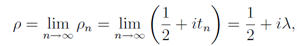 | (29) |
whereλ is real but tn is not necessarily a real number.[8]Now we think about the values of tn, which converge to a positive λ in the limit of n→∞ and put it into Eq.(16) | (30) |
Thus we write the solution to the equation 
 | (31) |
Using the n-th order relation of Eq.(21) | (32) |
we get the relation | (33) |
This form will be utilize to calculate zeros of the Riemann zeta function by way of the limit ofn→∞.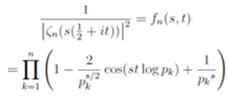 | (34) |
Here fn(s, t) and log fn(s, t) will diverge at the same time in n→∞, because fn(s, t)is positive. As all non-trivial zeros of the Riemann zeta function is expected on s =1, we study the following relation for s≥1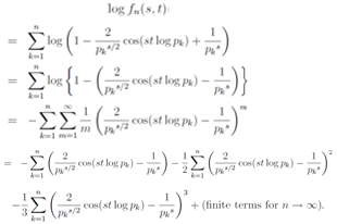 | (35) |
We regularize Eq.(35) in order to apply it even in the case s = 1. We try to regularize Eq.(35) by way of dividing an appropriate factor , which leaves a leading divergence divergent and makes a non-leading divergence convergent. In fact, we divide Eq.(35) by
 | (36) |
which we also adopted in the equation (26) of the first part.[7] Thus we study the divergence in the form of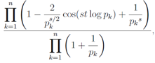 | (37) |
which corresponds in the summation form as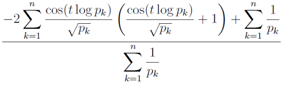 | (38) |
where we set s = 1. The leading divergent term of Eq.(38) in n→∞is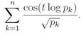 | (39) |
The form of divisor  means that using Mertens' theorem
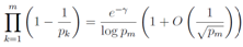 | (40) |
and the Euler's 
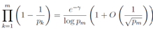 | (41) |
we get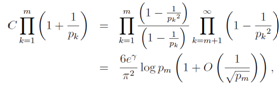 | (42) |
 | (43) |
where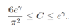 | (44) |
The Euler product representation for n→∞ is only valid for s≥2, and we restrict our interest for t>0. The zeros of the Riemann zeta function make Eq.(34) divergent, which means that products are multiplied maximally in the right hand side. Each term in Eq.(34) is maximized when  , namely,
 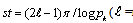 natural number). We give graphs for the superposition of cosine functions, which indicate the solution of
  as local maximum values,
 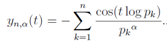 | (45) |
The graph of yn,α(t) for α =1/2 is printed as Figure 1, and judging from the graph of α =1 (Figure 2), the denominator pk seems to be well-matched to cancel the notches come from the superposition of cosine functions. Figure 1 is also such an example of notches. Figure 2 has the positive maximal values that correspond to the non-trivial zeros of the zeta function except the one appeared in t<6. Thus zeros of the Euler product representation in Eq.(34) preserve the value even in the form of the summation in Eq.(45).  | Figure 1. The graph of yn,αfor n =104 andα=1/2 |
 | Figure 2. The graph of yn,αfor n =106andα=1 |
The terms to regularize the divergence will be discussed, which is essential to the order on the critical line and seems to be closely related to the von Mangoldt function,[9] in a separate paper. On the other hand, the sum over the zeros of the zeta function for a certain prime p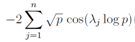 | (46) |
leads us a graph which indicates locations of the prime numbers.[3]
4. Nature of the Prime Numbers
Here we can show that the Riemann hypothesis holds for the L-function by using the approximate functional equation for the Dirichlet’sL-function as well as that by using the regularization for the Euler product as stated in part one. We listed the condition which leads a verificationalong these lines for the Riemann hypotheses as 1. the existence of the Euler product representation, 2. the prime number theorem  is satisfied, 3. the approximate functional equation of the Dirichlet’sL-function is satisfied. Exclusive uses of the Euler-Maclaurin expansion for the zeta function, which is actually an asymptotic expansion, have prevented the Riemann hypothesis from being demonstrated. According to the conclusion of the first part, the Riemann hypothesis for the Ramanujan’s zeta function or another zeta function is realized because each function has the Euler product representation. The Ramanujan’s conjecture for the Euler product corresponds the cosine term of the standard form for the Riemann zeta function, so it will hold because
  is less than one due to the independence of logpk’s. About the zeta functions, which have no non-trivial zero besides zeros of the Riemann hypotheses, we parametrize them to the standard form. In this case, the product of thezeros λj of the Riemann zeta function and log pk, the logarithm of the primes pk has a similar structure to θ of the Sato-Tate conjecture or the Sato-Tate theorem for the zeta function associated with the elliptical function proved by Richard Taylor. Moreover, in spite that theλj’s obey the uniform distribution to modulus one,[6] we claim that the response of j-direction increase(j =1, 2, ··· ,∞) forλj yields the similar distribution of the Sato-Tate conjecture,[11][16] once we takeλjlogpk to modulus 2π. The Sato-Tate conjecture claims that the response of k-direction increase(k =1, 2, ··· ,∞) for pk yields the distribution of
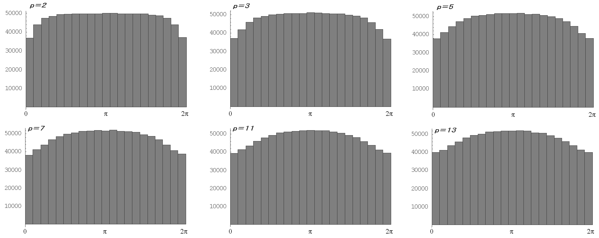 | Figure 3. The histograms(divided 21st) of distributions for pk= 2, 3, 5, 7, 11 and 13 beginning withj = 106 up to 2×10⁶ |
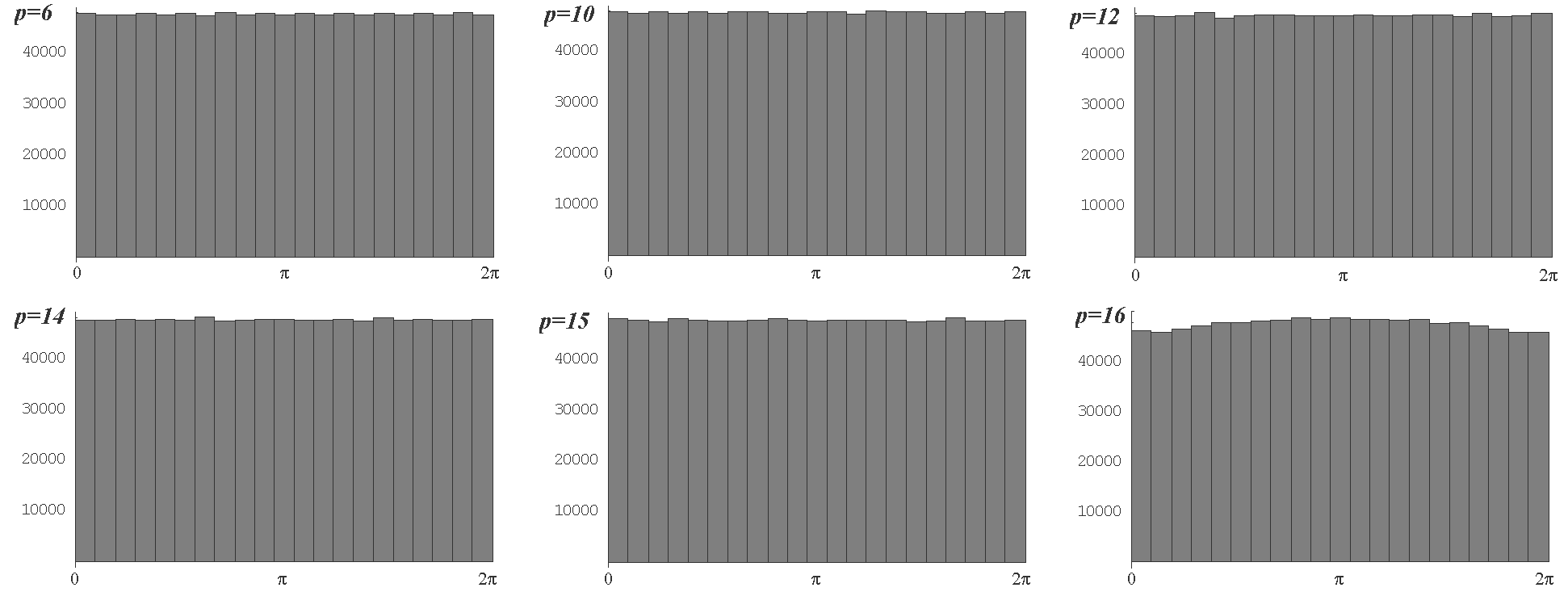 | Figure 4. The histograms(divided 21st) of distributions for p = 6, 10, 12, 14, 15 and 16 beginning withj = 106 up to 2×10⁶ |
 | (47) |
where  . On the other hand, once we put
  , we may claim that the response of j-direction increase ofλj yields the distribution of the Wigner’s semi-circle law, which is related by regarding
  of Eq.(47) as a single variable. Figure 3 is the histograms of distributions for pk= 2,3,5,7,11 and 13. In contrast to these histograms, the histograms of distributions in case that we put composite numbers(= 6,10,12,14,15 and 16) into pk, are also printed in Figure 4. In the cases for the power of one prime like p = 16, a shape of the peak around π slightly remains in the histogram, whereas the shape of the tales near 0 or 2π would be convex downwards.
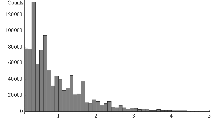 | Figure 5. The histogram(class interval = 0.1) for the distribution of the interval of pk/ log pk for 106 primes beginning with k = 106 |
A nature of primes is also found in a distribution for the interval of succeeding primes, | (48) |
where the logarithm terms exist in order to normalize to one. We present the histogram for 106 primes beginning with k = 106 in Figure 5 for example. The fluctuation in the histogram which rather looks like an oscillation never vanish for larger number of primes and is deeply related to the Wilson theorem and the Hoheisel's constant.[10]
5. Discussions and Remarks
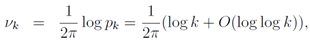
We discuss the equations which yield the primes and the zeros of the zeta functions in this section. We normalize the product of λjand log pkintroducing new notations μjand νkas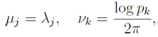 | (49) |
and the k-direction(k = 1, 2, ··· , ∞) average ofμjνk−1/2−[μjνk] will be 0 by the distribution like the Sato-Tate conjecture, where[ ] is the Gauss symbol. By the law of large number, we can write down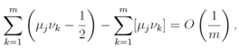 | (50) |
so we get 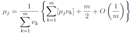 | (51) |
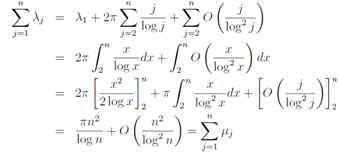
We can estimate the denominator as[15]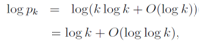 | (52) |
 | (53) |
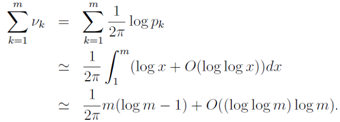 | (54) |
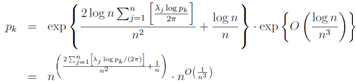
After all, we write a following approximate relation for anyμj,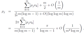 | (55) |
usingλj= μj,νk=log pk/(2π),we write the relation for any λj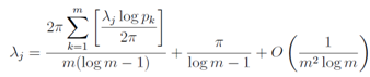 | (56) |
In the similar way,[12] we take the j-direction average ofμjνk−1/2−[μjνk], we can writedown by a symmetric property as illustrated in Figure 3, we get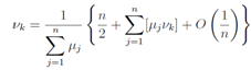 | (57) |
We also estimate the denominator as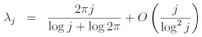 | (58) |
 | (59) |
so we write a following approximate relation for any νk,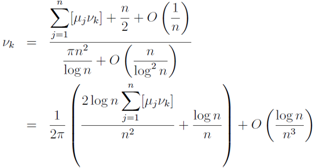 | (60) |
Finally we write down the relation for any pk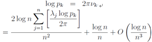 | (61) |
 | (62) |
Equations (56) and (62) are a set of equations which gives prime numbers and zeros of the Riemann zeta function.
References
| [1] | P. Borwein, S. Choi, B. Rooneyand A. Weirathmueller,The Riemann Hypothesis: A Resource for the Afficionado and Virtuoso Alike, CMS Books inMathematics, Springer- Verlag, 2008. |
| [2] | A. Connes and M. Marcolli, NoncommutativeGeometry, Quantum Fields and Motives, AMS, 2008. |
| [3] | J. B. Conrey, Figure 6 in ”The Riemann Hypothesis, Notice of the AMS,pp.341-353, 2003”. |
| [4] | J. B. Conrey, D. W. Farmer, J. P. Keating, M. O. Rubinstein and N. C. Snaith, Integral moments of L-functions, Proceedings of the London Mathematical Society 91, Cambridge University Press, pp.33-104, 2005. |
| [5] | C. P. Dettmann, New horizons in multidimensional diffusion: The Lorentz gas and the Riemann hypothesis. J.Stat. Phys. 146, pp.181-204, 2012. |
| [6] | P. D. T. A. Elliot, The Riemann zeta function and coin tossing, J. ReineAngew.Math. 254,pp.100-109, 1972. |
| [7] | M. Fujimoto and K. Uehara, Regularization for zeta functions with physical applications I, arXiv:math-ph/0609013, 2006. |
| [8] | M. Fujimoto and K. Uehara, A Brief Note on the Riemann Hypothesis I, II, arXiv:math-ph/0906.1099v2, 1003.2854, 2011. |
| [9] | A. Gut, Some remarks on the Riemann zeta distribution, Uppsala University Department of Mathematics Report, 2005. |
| [10] | G. Hoheisel, Primzahlprobleme in der Analysis, Berliner Sitzungsberichte, pp.580-588, 1930. |
| [11] | B. Mazur, Controlling our errors, Nature 443,pp.38-40, 2006. |
| [12] | A. Odlyzko, The 1020 -th Zero of the Riemann Zeta Function and 70 Million of the Neighbors, AT&T Bell Lab. Preprint, 1989. |
| [13] | D. Schumayer and D.A.W. Hutchinson, Colloquium: Physics of the Riemann hypothesis. Rev. Mod. Phys. 83, pp.307-330, 2011. |
| [14] | G. Sierra, A physics pathway to the Riemann hypothesis, arXiv:math-ph/1012.4264, 2010. |
| [15] | H. M. Srivastava and J.Choi, Series Associated with the Zeta and Related Function, Kluwer, 2001. |
| [16] | C. J.Swierczewski, Connections Between the Riemann Hypothesis and the Sato-Tate Conjecture, http//modular. math.washington.edu/projects/swierczewski.pdf, 2008. |
 Abstract
 Reference
 Full-Text PDF
 Full-Text HTML