| [1] | Goldhaber, G., and Perlmutter, S. 1998, A study of 42 type Ia supernovae and a resulting measurement of Omega(M) and Omega(Lambda). Physics Reports-Review Section of Physics Letters 307, 325–331. |
| [2] | Riess, A. G., Filippenko, A. V., Challis, P., and et al. 1998, Observational evidence from supernovae for an accelerating universe and a cosmological constant. Astron. J., 116, 1009–1038. |
| [3] | Garnavich, P. M., Kirshner, R. P., Challis, P., and et al. 1998, Constraints on cosmological models from Hubble Space Telescope observations of high-z supernovae. Astrophys. J. 493, L53+ Part 2. |
| [4] | Garnavich, P. M., Kirshner, R. P., Challis, P., and et al. 1998, Constraints on cosmological models from Hubble Space Telescope observations of high-z supernovae. Astrophys. J. 493, L53+ Part 2. |
| [5] | Volders, L. 1959, Neutral hydrogen in M 33 and M 101. Bulletin of the Astronomical Institutes of the Netherlands 14, 323–334. |
| [6] | De Blok, W. J. G., and McGaugh, S. 1997, The dark and visible matter content of low surface brightness disc galaxies. MNRAS 290, 533–552. |
| [7] | Clowe, D., Bradač, M., Gonzalez, A. H., Markevitch, M., Randall, S. W., Jones, C., and Zaritsky, D. 2006, A direct empirical proof of the existence of dark matter. Astrophys. J. 648, L109–L113. |
| [8] | Webb, J. K., Flambaum, V. V., Churchill, C. W., Drinkwater, M. J., and Barrow, J. D. 1999, Search for time variation of the fine structure constant. Phys. Rev. Lett. 82, 884–887. (arXiv:astro-ph/9803165) |
| [9] | Webb, J. K., Murphy, M. T., Flambaum, V. V., Dzuba, V. A., Barrow, J. D., Churchill, C. W., Prochaska, J. X., and Wolfe, A. M. 2001, Further evidence for cosmological evolution of the fine structure constant. Phys. Rev. Lett. 87, 091301. |
| [10] | Khatri, R., and Wandelt, B. D. 2007, 21-cm radiation: A new probe of variation in the fine-structure constant. Phys. Rev. Lett. 98, 111301. |
| [11] | Paal, G. 1970, The global structure of the universe and the distribution of quasi-stellar objects. Acta Phys. Acad. Sci. Hung. 30, 51–54. |
| [12] | Tifft, W. G. 1973, Properties of the redshift-magnitude bands in the Coma cluster. Astrophys. J. 179, 29–44. |
| [13] | Tifft, W. G. 2003, Redshift periodicities, the galaxy-quasar connection. Astrophys. Space Sci. 285, 429–449. |
| [14] | Carnot, S. 1824, Reflexions sur la puissance motrice du feu et sur les machines propres a developper cette puissance. Bachelier, Paris. |
| [15] | Jaynes, E. T. 2003, Probability theory. The logic of science. Cambridge University Press, Cambridge, UK. |
| [16] | Sharma, V., and Annila, A. 2007, Natural process – Natural selection. Biophys. Chem. 127, 123–128. |
| [17] | Du Châtelet, E. 1740, Institutions de physique. Paris, France: Prault. Facsimile of 1759 edition Principies mathématiques de la philosophie naturelle I-II. Éditions Jacques Gabay, Paris. |
| [18] | ‘s Gravesande, W. 1720, Physices elementa mathematica, experimentis confirmata, sive introductio ad philosophiam Newtonianam. Leiden, The Netherlands. |
| [19] | Jaakkola, S., Sharma, V., and Annila, A. 2008, Cause of chirality consensus. Curr. Chem. Biol. 2, 53–58. (arXiv:0906.0254) |
| [20] | Jaakkola, S., El-Showk, S., and Annila, A. 2008, The driving force behind genomic diversity. (arXiv:0807.0892) |
| [21] | Grönholm, T., and Annila, A. 2007, Natural distribution. Math. Biosci. 210, 659–667. |
| [22] | Würtz, P., and Annila, A. 2008, Roots of diversity relations. J. Biophys. (doi:10.1155/2008/654672) (arXiv:0906.0251) |
| [23] | Annila, A., and Annila, E. 2008, Why did life emerge? Int. J. Astrobiol. 7, 293–300. |
| [24] | Annila, A., and Kuismanen, E. 2008, Natural hierarchy emerges from energy dispersal. BioSystems 95, 227–233. |
| [25] | Karnani, M., and Annila, A. 2009, Gaia again. BioSystems 95, 82–87. |
| [26] | Sharma, V., Kaila, V. R. I., and Annila, A. 2009, Protein folding as an evolutionary process. Physica A 388, 851–862. |
| [27] | Würtz, P., and Annila, A. 2010, Ecological succession as an energy dispersal process. BioSystems 100, 70–78. |
| [28] | Annila, A., and Salthe, S. 2009, Economies evolve by energy dispersal. Entropy 11, 606–633. |
| [29] | Annila, A. 2011, Least-time paths of light. MNRAS 416, 2944–2948. |
| [30] | Koskela, M., and Annila, A. 2011, Least-time perihelion precession. MNRAS 417, 1742–1746. |
| [31] | Tuisku, P., Pernu, T. K., and Annila, A. 2009, In the light of time. Proc. R. Soc. A. 465, 1173–1198. |
| [32] | Annila, A. 2010, The 2nd law of thermodynamics delineates dispersal of energy. Int. Rev. Phys. 4, 29–34. |
| [33] | Kaila, V. R. I., and Annila, A. 2008, Natural selection for least action. Proc. R. Soc. A. 464, 3055–3070. |
| [34] | Annila, A. 2010, All in action. Entropy 12, 2333–2358. |
| [35] | Eddington, A. S. 1928, The nature of physical world. MacMillan, New York, NY. |
| [36] | Gibbs, J. W. 1993–1994, The scientific papers of J. Willard Gibbs. Ox Bow Press, Woodbridge, CT. |
| [37] | Wyld, H. W. 1961, Formulation of the theory of turbulence in an incompressible fluid. Ann. Phys. 14, 143–165. |
| [38] | Keldysh, L. V. 1964, Zh. Eksp. Teor. Fiz. 47, 1515–1527; 1965 Diagram technique for nonequilibrium processes. Sov. Phys. JETP 20, 1018–1026. |
| [39] | Boltzmann, L. 1905, Populäre Schriften. Barth, Leipzig, Germany. [Partially transl. Theoretical physics and philosophical problems by B. McGuinness, Reidel, Dordrecht 1974.] |
| [40] | De Donder, Th. 1936, Thermodynamic theory of affinity: A book of principles. Oxford University Press, Oxford, UK. |
| [41] | Kullback, S. 1959, Information theory and statistics. Wiley, New York, NY. |
| [42] | Salthe, S. N. 2002, Summary of the principles of hierarchy theory. General Systems Bulletin 31, 13–17. |
| [43] | Salthe, S. N. 2007, The natural philosophy of work. Entropy 9, 83–99. |
| [44] | Noether, E. 1918, Invariante Variationprobleme. Nach. v.d. Ges. d. Wiss zu Goettingen, Mathphys. Klasse 235–257; English translation Tavel, M. A. 1971 Invariant variation problem. Transp. Theory Stat. Phys. 1, 183–207. |
| [45] | Jaynes, E. T. 1957, Information theory and statistical mechanics. Phys. Rev. 106, 620–630. |
| [46] | Roshdi, R. 1992, Optique et Mathematiques: Recherches sur L’Histoire de la Pensee Scientifique en Arabe. Variorum, Aldershot, UK. |
| [47] | Lotka, A. J. 1922, Natural selection as a physical principle. Proc. Natl. Acad. Sci. 8, 151–154. |
| [48] | Zinn-Justin, J. 2002, Quantum field theory and critical phenomena. Oxford University Press, New York, NY. |
| [49] | Peskin, M., and Schroeder, D. 1995, An introduction to quantum field theory. Philadelphia, PA: Westview Press. |
| [50] | Thirring, W. 1970, Systems with negative specific heat. Z. Physik 235, 339– 352. |
| [51] | Pokorski, S. 1987, Gauge field theories. Cambridge University Press. Cambridge, UK. |
| [52] | Darwin, C. 1859, On the origin of species. John Murray, London, UK. |
| [53] | Penzias, A. A., and Wilson R. W. 1965, A measurement of excess antenna temperature at 4080 Mc/s. Astrophys. J. 142, 419–421. |
| [54] | Karnani, M., Pääkkönen, K., and Annila, A. 2009, The physical character of information. Proc. R. Soc. A. 465, 2155–2175. |
| [55] | Poynting, J. H. 1920, Collected scientific papers. Cambridge University Press, London. |
| [56] | Lavenda, B. H. 1985, Nonequilibrium statistical thermodynamics. John Wiley and Sons, New York, NY. |
| [57] | Gouy, L. G. 1889, Sur l'energie utilizable. J. de Physique 8, 501–518. |
| [58] | Stodola, A. 1910, Steam and gas turbines. McGraw-Hill, New York, NY. |
| [59] | Weinberg, S. 1972, Gravitation and cosmology, principles and applications of the general theory of relativity. Wiley, New York, NY. |
| [60] | Berry, M. 2001, Principles of cosmology and gravitation. Cambridge University Press, Cambridge, UK. |
| [61] | Taylor, E. F., and Wheeler, J. A. 1992, Spacetime physics. Freeman, New York, NY. |
| [62] | Lorenz, L. 1867, On the identity of the vibrations of light with electrical currents. Philos. Mag. 34, 287–301. |
| [63] | Einstein, A. 1905, On the electrodynamics of moving bodies. Annalen der Physik 17, 891–921. |
| [64] | Connes, A. 1994, Noncommutative geometry (Géométrie non commutative). Academic Press, San Diego, CA. |
| [65] | Lemaître, G. 1927, Un univers homogène de masse constante et de rayon croissant rendant compte de la vitesse radiale des nébuleuses extra-galactiques. Annales de la Société Scientifique de Bruxelles 47, 49–56. |
| [66] | Hubble, E. 1929, A relation between distance and radial velocity among extra-galactic nebulae. Proc. Natl. Acad. Sci. USA 15, 168–173. |
| [67] | Hawking, S. W. 1974, Black hole explosions. Nature 248, 30–31. |
| [68] | Sciama, D. W. 1953, On the origin of inertia. MNRAS 113, 34–42. |
| [69] | Dicke, R. H. 1961, Dirac's cosmology and Mach's principle. Nature 192, 440–441. |
| [70] | Haas, A. 1936, An attempt to a purely theoretical derivation of the mass of the universe. Phys. Rev. 49, 411–412. |
| [71] | Tryon, E. P. 1973, Is the universe a vacuum fluctuation? Nature 246, 396–397. |
| [72] | Planck, M. 1899, Über irreversible Strahlungsvorgänge. Sitzungsberichte der Königlich Preußischen Akademie der Wissenschaften zu Berlin 5, 440–480. |
| [73] | Bennett, C.L. et al., 2003, First-year Wilkinson Microwave Anisotropy Probe (WMAP) Observations: Preliminary maps and basic results. Astrophys. J. Suppl. Series, 148, 1–27. |
| [74] | Salthe, S. N. 1985, Evolving hierarchical systems: Their structure and representation. Columbia University Press, New York, NY. |
| [75] | Tully, R. B., and Fisher, J. R. 1977, A new method of determining distances to galaxies. Astronomy and Astrophysics 54, 661–673. |
| [76] | Milgrom, M. 1983, A modification of the Newtonian dynamics as a possible alternative to the hidden mass hypothesis. Astrophys. J. 270, 365–370. |
| [77] | Anderson, J. D., Laing, P. A., Lau, E. L., Liu, A. S., Nieto, M. M., and Turyshev, S. G. 1998, Indication, from Pioneer 10/11, Galileo, and Ulysses data, of an apparent anomalous, weak, long-range acceleration. Phys. Rev. Lett. 81, 2858–2861. |
| [78] | Bertolami, O., and Páramos, J. 2004, Pioneer's Final Riddle. arXiv:gr-qc/0411020. |
| [79] | Anderson, J. D., and Nieto, M. M. 2009, Astrometric solar-system anomalies. In Relativity in Fundamental Astronomy. Proceedings IAU Symposium No. 261, Klioner, S. A., Seidelman, P. K., and Soffel, M. H. eds. arXiv:0907.2469v2. |
| [80] | Francisco, F., Bertolami, O., Gil, P. J. S., and Páramos J. 2011, Modelling the reflective thermal contribution to the acceleration of the Pioneer spacecraft. arXiv:1103.5222. |
| [81] | Koschmieder, E. L. 1993, Bénard cells and Taylor vortices. Cambridge University Press, New York, NY. |
| [82] | Taylor, G. I. 1923, Stability of a viscous liquid contained between two rotating cylinders. Phil. Trans. R. Soc. A 223, 289–343. |
| [83] | Feynman, R. P. 1955, Application of quantum mechanics to liquid helium. Prog. Low Temp. Phys. 1, 17–53. |
| [84] | De Maupertuis, P.-L. M. 1744, Accord de différentes loix de la nature qui avoient jusqu’ici paru incompatibles. Mém. Ac. Sc. Paris 417–426. |
| [85] | Clemence, G. M. 1947, The relativity effect in planetary motions. Rev. Mod. Phys. 19, 361–364. |
| [86] | Zwicky, F. 1933, Die Rotverschiebung von extragalaktischen Nebeln. Helvetica Physica Acta 6, 110–127. |
| [87] | Zwicky, F. 1937, On the masses of nebulae and of clusters of nebulae. Astrophys. J. 86, 217–246. |
| [88] | Charlton, J. C., and Schramm, D. N. 1986, Percolation of explosive galaxy formation. Astrophys. J. Part 1 310, 26. |
| [89] | Bok, B. J., and Reilly, E. F. 1947, Small dark nebulae. Astrophys. J. 105, 255–257. |
| [90] | Annila, A. 2011, Physical portrayal of computational complexity. ISRN Computational Mathematics (in press) (www.isrn.com/journals/cm/aip/321372/) (arXiv:0906.1084) |
| [91] | Poincaré, J. H. 1890, Sur le problème des trois corps et les équations de la dynamique. Divergence des séries de M. Lindstedt. Acta Mathematica 13, 1–270. |
| [92] | Strogatz, S. H. 2000, Nonlinear dynamics and chaos with applications to physics, biology, chemistry and engineering. Westview, Cambridge, MA. |
| [93] | Newman, J. R. 1956, The world of mathematics. Simon and Schuster, New York, NY. |
| [94] | www.claymath.org/millennium/Navier-Stokes_Equations/ |
| [95] | Van Moerbeke, P. 1989, Introduction to algebraic integrable systems and their Panlevé analysis. Proceeding of Symposia in Pure Mathematics 49. |
| [96] | Pernu, T. K., and Annila, A. 2012, Natural emergence. Complexity. (in press) |
| [97] | Mackay, A. L. 1977, The harvest of a quiet eye - a selection of scientific quotations. Bristol, UK: The Institute of Physics. |
| [98] | Kondepudi, D., and Prigogine, I. 1998, Modern thermodynamics. Wiley, New York, NY. |
| [99] | Verhulst, P. F. 1845, Recherches mathématiques sur la loi d’accroissement de la population. Nouv. Mém. Acad. Roy. Sci. Belleslett. Bruxelles 18, 1–38. |
| [100] | May, R. M. 1976, Simple mathematical models with very complicated dynamics. Nature 261, 459–467. |
| [101] | Waage, P., and Guldberg, C. M. 1864, Forhandlinger 35 Videnskabs-Selskabet i Christiana. |
| [102] | Cooley, J. W., and Tukey, J. W. 1965, An algorithm for the machine calculation of complex Fourier series. Math. Comput. 19, 297–301. |
| [103] | Lehto, A. 2009, On the Planck scale and properties of matter. Nonlinear Dyn. 55, 279–298. |
| [104] | Alonso, M., and Finn, E. J. 1983, Fundamental university physics. 3. Addison-Wesley, Reading, MA:. |
| [105] | Ryden, B. 2003, Introduction to cosmology. Addison-Wesley, New York, NY. |
| [106] | Crawford, F. S. 1968, Waves in Berkeley physics course. 3. McGraw-Hill, New York, NY. |
| [107] | Tifft, W. G. 1996, Global redshift periodicities and periodicity structure. Astrophys. J. 468, 491–518. |
| [108] | Napier, W. M. 2003, A statistical evaluation of anomalous redshift claims. Astrophys. Space Sci. 285, 419–427. |
| [109] | Chwolson, O. 1924, Über eine mögliche Form fiktiver Doppelsterne. Astronomische Nachrichten 221, 329–330. |
| [110] | Einstein, A. 1936, Lens-like action of a star by the deviation of light in the gravitational field. Science 84, 506–507. |
| [111] | Rosen, K. H. 1993, Elementary number theory and its applications. Reading, MA: Addison-Wesley. |
| [112] | Schramm, W. 2008, The Fourier transform of functions of the greatest common divisor. Integers 8, A50. |
| [113] | Richman, F. 1971, Number theory: An introduction to algebra. Wadsworth, Belmont, CA. |
| [114] | Feynman, R., Leighton, R. B., and Sands, M. 1963, The Feynman lectures on physics. Addison-Wesley, Reading, MA. |
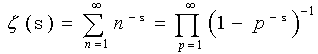
| [115] | Erickson, C. 2005, A geometric perspective on the Riemann zeta function’s partial sums. SURJ Mathematics 22–31. |
| [116] | Bernoulli, J. 1967, Opera, Tomus Secundus. Brussels, Belgium: Culture et Civilisation. |
| [117] | Mäkelä, T., and Annila, A. 2010, Natural patterns of energy dispersal. Phys. Life. Rev. 7, 477–498. |
| [118] | Hardy, G. H., and Littlewood, J. E. 1921, The zeros of Riemann’s zeta function on the critical line. Math. Z. 10, 283–317. |
| [119] | Titchmarsh, E. C. 1986, The theory of the Riemann zeta function. Oxford Science Publications, Oxford, UK. |
| [120] | www.claymath.org/millennium/Riemann_Hypothesis/ |
| [121] | Golub, G. H., and Van Loan, C. F. 1996, Matrix computations. The Johns Hopkins University Press, Baltimore, MD. |
| [122] | Franel, J., and Landau, E. 1924, Les suites de Farey et le problème des nombres premiers. Göttinger Nachr. 198–206. |
| [123] | Montgomery, H. L. 1973, The pair correlation of zeros of the zeta function. Analytic number theory, Proc. Sympos. Pure Math., XXIV, 181–193. Providence, RI: Am. Math. Soc. |
| [124] | Berry, M. V., and Keating, J. P. 1999, H = xp and the Riemann zeros. Supersymmetry and trace formulae: Chaos and disorder. 355–367 eds. Keating, J. P., Khmelnitski, D. E., and Lerner, I. V. Plenum, New York, NY. |
| [125] | Spector, D. 1990, Supersymmetry and the Möbius inversion function. Commun. Math. Phys. 127, 239–252. |
| [126] | Silverman, J. H. 1992, The arithmetic of elliptic curves. Springer-Verlag, New York, NY. |
| [127] | Lang, S. 1992, Algebra. Addison-Wesley, Reading, MA. |
| [128] | www.claymath.org/millennium/Birch_and_Swinnerton-Dyer_Conjecture/ |
| [129] | Tate, J. 1974, The arithmetic of elliptic curves. Invent. Math. 23, 179–206. |
| [130] | Eddington, A. S. 1931, Preliminary note on the masses of the electron, the proton and the Universe. Proc. Camb. Phil. Soc. 27, 15–19. |
| [131] | Dirac, P. A. M. 1938, A new basis for cosmology. Proc. R. Soc. A 165, 199–208. |
| [132] | Barrow, J. D., and Tipler, F. J. 1986, The anthropic cosmological principle. Oxford University Press, New York, NY. |
| [133] | Klein, M. J. 1967, Thermodynamics in Einstein’s thought. Science 157, 509–516. |
 Abstract
 Reference
 Full-Text PDF
 Full-text HTML

 ,
, ] = px – xp = –iħ. This form corresponding to 2Kt + Ut = Qt of an incoherent system follows from the quantized least action (∂/∂t)(
  ) = 0 using the expectation values ∂
 /∂t = –∂U/∂x for the momentum
  = –iħ∂/∂x and coordinate
  = x and energy
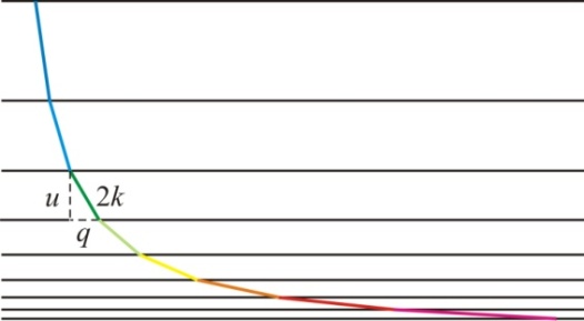
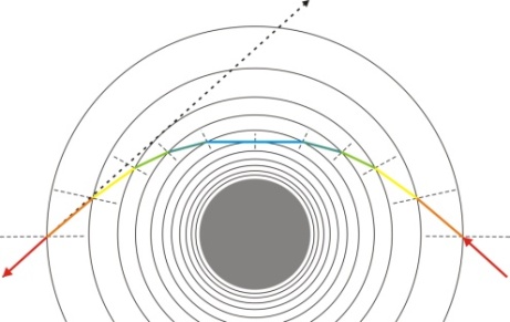
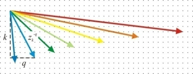
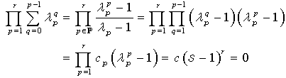
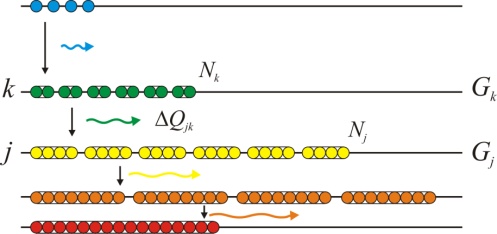
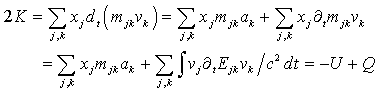
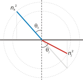
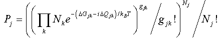
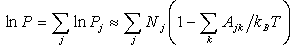
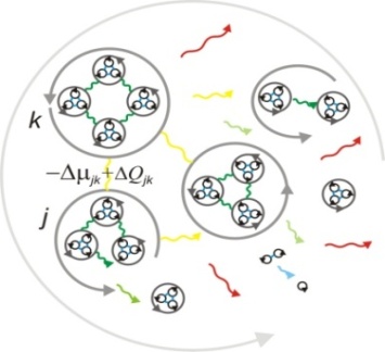
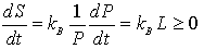
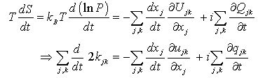
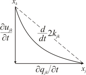
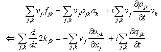
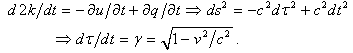
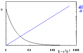
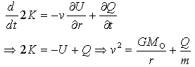
 = –iħ∂/∂t operators. Transformations with net dissipation are non-commutative, but when to-and-fro flows cancel each other exactly over the integration period, the system remains Hamiltonian, e.g., given by Liouville-von Neumann equation. Therefore the solutions are available by a unitary transformation to a time-independent frame which is in fact the signature of a stationary state. Operator algebra is a convenient way to track the relative phases of coherence pathways but it does not, as such, bring forward new evolutionary phenomena. Thus we prefer the basic formalism (Eqs. 2.1 – 2.4) to study the proposed galactic red-shift clustering and eventual variation in the fine-structure constant.The initial state of the Universe at the ultraviolet fixed point is pictured by Eq. 2.1 as an elemental system N1 = 1 composed of indistinguishable basic entities in degenerate numbers N0 = g10. The energy difference G10 = G1 – G0 = kBT between the nascent Universe and its “surroundings” at zero density G1 = 0 is huge. The initial probability (Eq. 2.1) P = [N0exp(–G10/kBT)]g10/g10! is the natural starting point for a series of transformations to increase P in least time.The Universe will evolve by lowering its degeneracy from g10 by spontaneous symmetry breaking. In phase transitions the basic entities will transform (combine) to diverse and distinct constituents in numbers Nk>0. Concomitantly G10 will fracture to diverse scalar Gjk and vector Qjk potential differences. In other words, the high factorials and energy differences of the nascent improbable state are conquered by divisions as soon as possible. Recursive decimation-in-time by two is the familiar example from the fast Fourier transformation[102]. However the general principle does not expose particular mechanisms of dispersal, but the flows will naturally select those to disperse energy in least time. Independent of the short-scale dynamics the universal process is bound asymptotically to Pmax. At the ultimate equilibrium i.e., at the infrared fixed point all densities will vanish (kBT → 0).According to the step-by-step evolution, the Universe is an expanding resonator (cavity) where energy is dispersing to lower and lower harmonics[103]. The expression of propagating waves as a sum of standing waves subject to boundary conditions is familiar from the derivation of Planck’s law[104]. During early epochs when the universal index of refraction n was high, photons were not effective in dispersal until recombination[105] since high-energy fluxes suffer more than low-energy fluxes from internal reflections at boundaries. Therefore, to inflate in least time, the natural selection for the maximal dispersal might have favored some primordial dissipative mechanisms other than photons. When the “surroundings” is at zero density, the condition of the maximal transmission in a stratified medium[106] is the geometric mean (√n) which implies a power-series reduction (Figure 5). A series in powers of two has been proposed to account for the quantized red-shifts of 21-cm lines recorded from distant galaxies[103,107,108].