-
Paper Information
- Paper Submission
-
Journal Information
- About This Journal
- Editorial Board
- Current Issue
- Archive
- Author Guidelines
- Contact Us
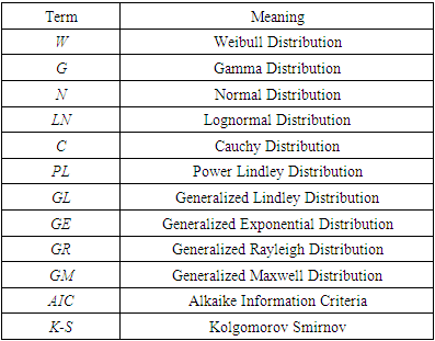
International Journal of Probability and Statistics
p-ISSN: 2168-4871 e-ISSN: 2168-4863
2022; 11(1): 19-27
doi:10.5923/j.ijps.20221101.03
Received: Nov. 16, 2022; Accepted: Dec. 19, 2022; Published: Dec. 28, 2022

Estimation of Wind Power Using a New Two Variable Copula-based Model in South Eastern Nigeria
 Abstract
 Reference
 Full-Text PDF
 Full-text HTML
Opabisi Adeyinka Kosemoni1, Adeyemo Samuel O.1, Ohaegbulam Promise O.2
1Department of Mathematics/Statistics, Federal Polytechnic Nekede, Owerri, Imo State, Nigeria
2Department of Food Technology, Federal Polytechnic Nekede, Owerri, Imo State, Nigeria
Correspondence to: Opabisi Adeyinka Kosemoni, Department of Mathematics/Statistics, Federal Polytechnic Nekede, Owerri, Imo State, Nigeria.
| Email: |  |
Copyright © 2022 The Author(s). Published by Scientific & Academic Publishing.
This work is licensed under the Creative Commons Attribution International License (CC BY).
http://creativecommons.org/licenses/by/4.0/

This study examines the use of other probability models as alternative for modeling wind speed data. The 2-parameter Weibull distribution is usually taken as the conventional model for fitting and analyzing wind speed observations. However, within the vanguard of statistical modeling, there exist other probability models which can also serve this purpose. In this paper, a study on ten probability models which can be used to fit wind speed observation is carried out. The models include: the Weibull, normal, Cauchy, gamma, power Lindley, generalized Lindley, generalized Rayleigh, generalized Maxwell, lognormal and the generalized exponential distributions. All ten models were used to fit monthly average wind speed observations from South-East Nigeria for the period (1987 – 2019). Results from the analysis showed that while the Weibull model remains a dominant model for the wind regime, the power Lindley and the normal distributions offered a very suitable alternative as well, as they offered very good fits to the wind speed observation which are indicative by their respective AIC, K-S and P-values.
Keywords: Goodness-of-fit Measures, Maximum Likelihood, Parameters, Probability Distributions, Wind Speed
Cite this paper: Opabisi Adeyinka Kosemoni, Adeyemo Samuel O., Ohaegbulam Promise O., Estimation of Wind Power Using a New Two Variable Copula-based Model in South Eastern Nigeria, International Journal of Probability and Statistics , Vol. 11 No. 1, 2022, pp. 19-27. doi: 10.5923/j.ijps.20221101.03.
Article Outline
1. Introduction
- Within the practice of wind speed modeling, the 2-parameter Weibull distribution with shape and scale parameters has been used more or less as the conventional wind speed model of which have been explored by several scholars. This has been due to the fact that the Weibull model covers a wide range of the shape of most wind regime because of the flexibility inherent in its density [10]. However, other models have also been suggested and used in many studies as alternative to the Weibull model depending on the wind regime that is being studied. Examples of such models include: the Rayleigh, Burr XII, gamma, inverse gamma, normal, inverse normal, exponential, log-normal, exponentiated Weibull, log-logistics, Pearson V, Pearson VI and the uniform distributions. The main reason for these studies has been to obtain the most appropriate theoretical wind speed distribution of a particular location or wind regime. In this paper, a study of ten wind speed model is undertaken using data from South-East Nigeria which lies on a low wind speed zone. The Weibull distribution alongside the normal, Cauchy, gamma, power Lindley, generalized Lindley, generalized Rayleigh, generalized Maxwell, lognormal and the generalized exponential distributions are used to fit wind speed sample from the zone and the results compared using some statistical goodness-of-fit measures. These distributions are two variable models with some being special cases of some extended distributions [21]. The rest of the paper is organized as follows. In section 2 the ten wind speed models considered are specified by their cumulative distribution function (cdf) and their probability density function (pdf). A description of the data used for the study and the analytical tools of analysis are contained in section 3. Section 4 contains the results obtained from the study. The paper closes in section 5 with summary and conclusion.
2. Wind Speed Models
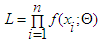
- Here we specify the cdfs and the pdfs of the various wind speed models considered in the study. The functional form of the Weibull model is used to begin the section.
2.1. Weibull Distribution (W)
- The cdf and pdf of the Weibull distribution are given respectively by
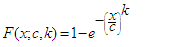 | (1) |
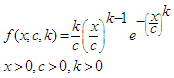 | (2) |
2.2. Gamma Distribution (G)
- The gamma distribution has cdf and pdf defines respectively as
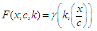 | (3) |
 | (4) |
 and
and  are the gamma and lower incomplete gamma functions respectively. The parameters c and k are scale and shape parameters respectively. For k=1, the distribution becomes the exponential distribution [16].
2.3. Normal Distribution (N)
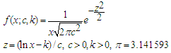
- The normal distribution is the most important distribution in statistical theory. It has cdf and pdf given respectively by
 | (5) |
 | (6) |
 is the lower incomplete gamma function. The positive sign in
  is valid for
  and the negative sign for
  . The parameters k and c are the mean (location parameter) and standard deviation (scale parameter) of the distribution respectively [17].
2.4. Lognormal Distribution (LN)
- The lognormal distribution is the distribution of a random variable whose logarithm is normally distributed. It has cdf and pdf expressed respectively by
 | (7) |
 | (8) |
 is the lower incomplete gamma function. The positive sign in
  is valid for
  and the negative sign for
  . The parameters
  and C are the location and scale parameters of the distribution respectively [17].
2.5. Cauchy Distribution (C)
- The Cauchy distribution also known as the Cauchy – Lorentz distribution, is the distribution of the ratio of two independent normally distributed random variables with zero means. It has cdf and pdf given respectively by
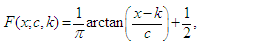 | (9) |
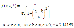 | (10) |
 and C are the location and scale parameters of the distribution respectively [17].
2.6. Power Lindley Distribution (PL)
- The power Lindley distribution was developed by Ghitany et al. [18]. It has cdf and pdf given by
 | (11) |
 | (12) |
 the distribution becomes the Lindley distribution.
2.7. Generalized Lindley Distribution (GL)
- The generalized Lindley distribution was proposed by Nadarajah et al. [19] with cdf and pdf expressed respectively as
 | (13) |
 | (14) |
 and
and  are scale and shape parameters respectively and for
  the distribution becomes the Lindley distribution.
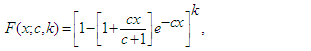
2.8. Generalized Exponential Distribution (GE)
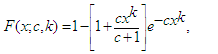
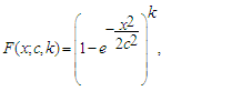
- The generalized exponential distribution was defined by Gupta and Kundu [20] as an alternative distribution to the Weibull distribution. The cdf and pdf of the distribution is expressed respectively as
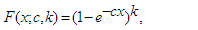 | (15) |
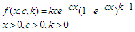 | (16) |
 and
and  are scale and shape parameters respectively and for k=1 the distribution becomes the exponential distribution.
2.9. Generalized Rayleigh Distribution (GR)
- The generalized Rayleigh distribution is a generalization of the 1-parameter Rayleigh distribution through the addition of a shape parameter. The cdf and pdf of the distribution is given respectively by
 | (17) |
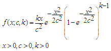 | (18) |
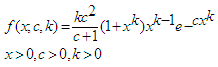
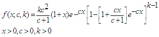
2.10. Generalized Maxwell Distribution (GM)
- The generalized Maxwell distribution is an extension of the 1-parameter Maxwell distribution through the addition of a scale parameter. The cdf and pdf of the distribution are given respectively by
 | (19) |
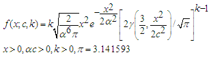 | (20) |
 is a scale parameter,
  is shape parameter and
  is the lower incomplete gamma function [17]. For
  , the distribution becomes the Rayleigh distribution.
3. Data and Analytical Tools
- The analysis is based on 33 years (1987- 2019) monthly average wind speed observations obtained from South-East Nigeria. The wind speed observations were obtained at a height of 10m with 384 sample observations. The highest and lowest wind speed observations are 5.8m/s and 0.7m/s respectively and this indicates that the region lies on the low wind speed zone in Nigeria. The mean wind speed is 3.59m/s, while the median wind speed is 3.60m/s The coefficient of skewness is -0.12 which clearly indicates that the distribution of the wind speed observation is skewed to the left. Also, the coefficient of excess kurtosis is -0.36 which implies that the distribution of the wind speed is light-tailed. Figure 1 shows the trend plot of the wind speed observation. The actual wind speed sample can be made available upon request from the corresponding author.
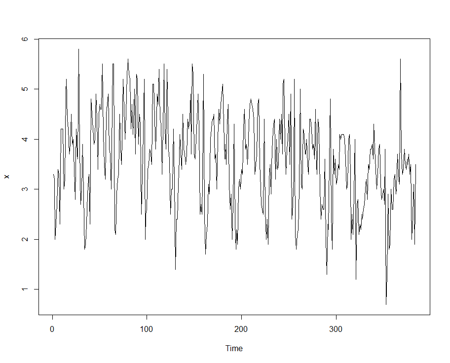 | Figure 1. The monthly average wind speed observation from South-East Nigeria (1987-2019) |
 | (21) |
 | (22) |
 | (23) |
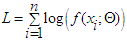
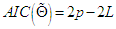
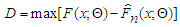
 is the maximum likelihood estimator of the parameter vector Θ, p is the number of parameters in the parameter vector Θ and L is the value of the log-likelihood. Among several competing distributions, the one with the smallest AIC value is considered the best model for the data set. The Kolmogorov-Smirnov (K-S) statistic is one of the most useful non-parametric test statistics in statistical literature. The statistic is obtained by making use of ranks of the wind speed observations. The K-S test statistic is used to compare a theoretical cumulative distribution function
  of a continuous random variable X to an empirical cumulative distribution function (ECDF)
  of a random sample of size n. The ECDF is based on the order statistics
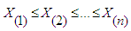 | (24) |
 denoting the order statistic. The ECDF
  is defined as the number of data points less than or equal to x divided by the sample size n. It can be expressed in terms of the order statistics as
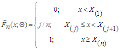 | (25) |
 | (26) |
 and an alternative hypothesis
  for a given
  level of significance. Under
  while
while  specifies that
 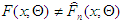 . The distribution of the observed sample is taken to be the same as that of the theoretical distribution
  (i.e.
(i.e.  is true) if
  where
where  is the tabulated critical value for the given
  level of significance. Associated with the K-S statistic is a quantity called the p-value which is sometimes referred to as the observed level of significance. The p-value is defined as the probability of observing a value of the test statistic
  as extreme as or more extreme than the one that is observed, when
  is true. A p-value less than or equal to the given
  level of significance will lead to the rejection of
  . In this paper we took
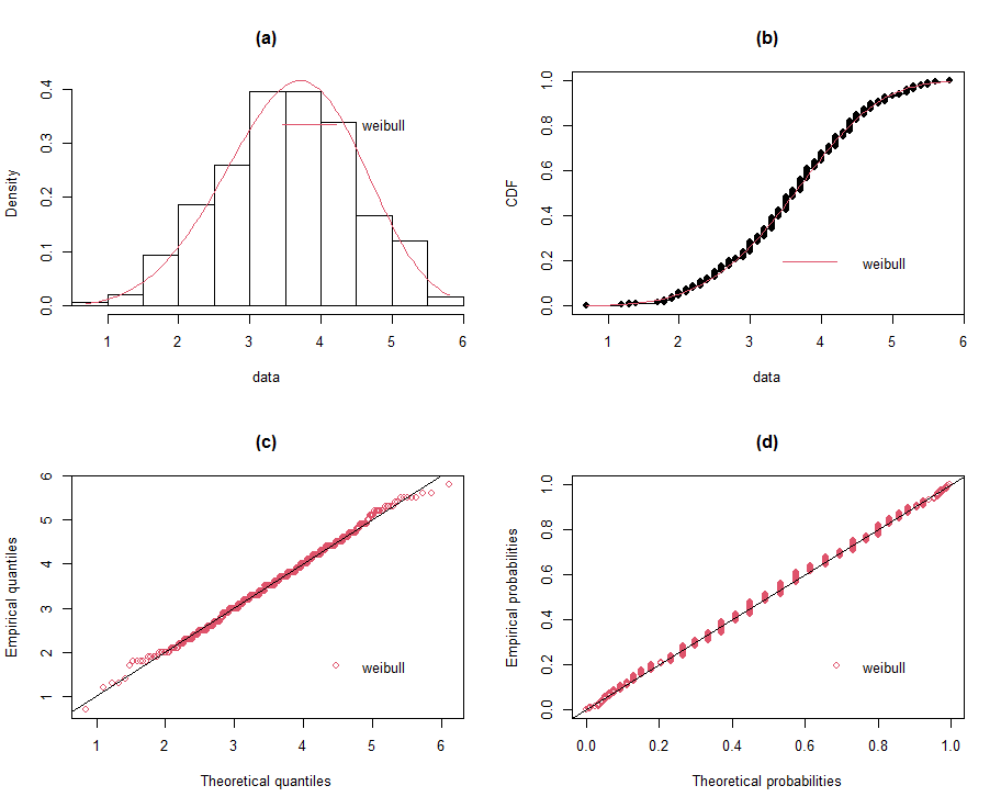
  . Also, the distribution with the highest p-value of the K-S statistic value is adjudged as the best in fitting the wind speed observation. The density plots which compare the histograms of the data and the fitted densities, the cumulative distribution function plots which compare the ECDF of the data and the fitted cdfs, the Q-Q plots which compare the empirical quantiles and the theoretical quantiles of the fitted distributions and the P-P plots which compare the empirical probabilities and the theoretical probabilities of the fitted distributions for all the fitted distributions were also generated and used in assessing the performance of all the distributions in fitting the wind speed observations.
 4. Results
- The results of parameter estimates of the ten distributions are contained Table 1 with their respective AIC, K-S and p-values.
|
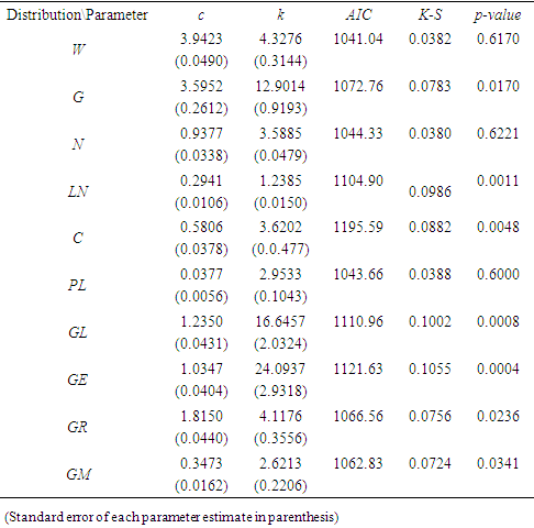
 | Figure 2 (a-d). Fitted Weibull distribution |
 | Figure 3 (a-d). Fitted gamma distribution |
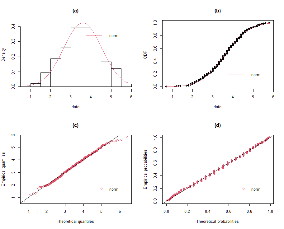 | Figure 4 (a-d). Fitted normal distribution |
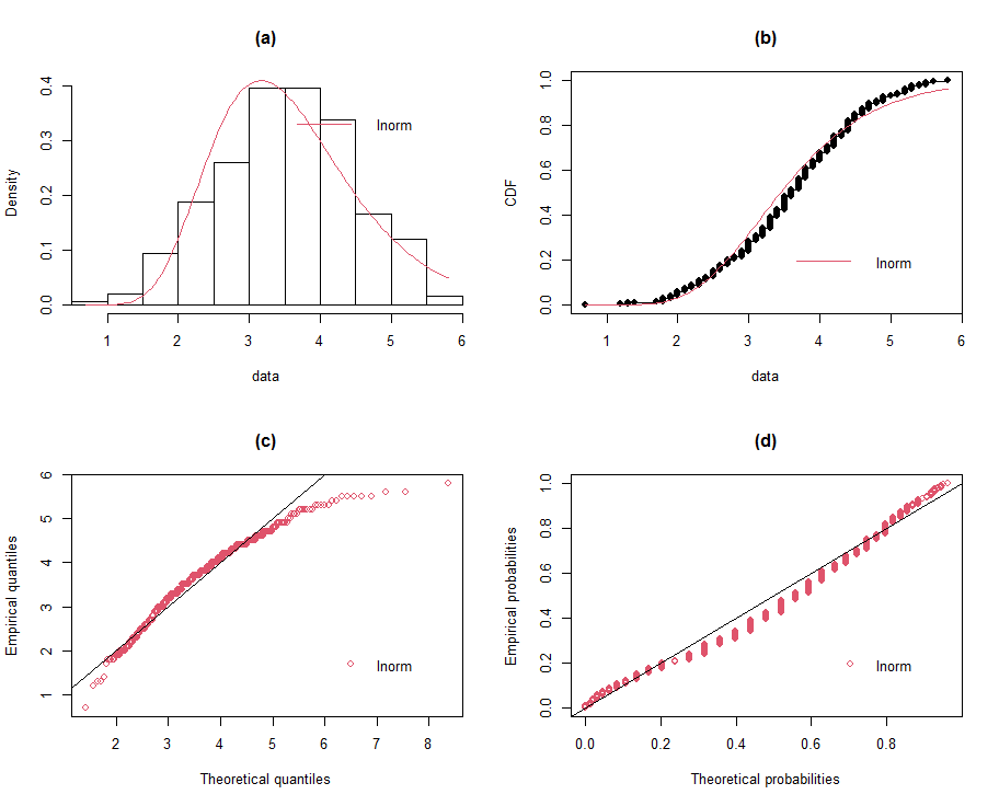 | Figure 5 (a-d). Fitted lognormal distribution |
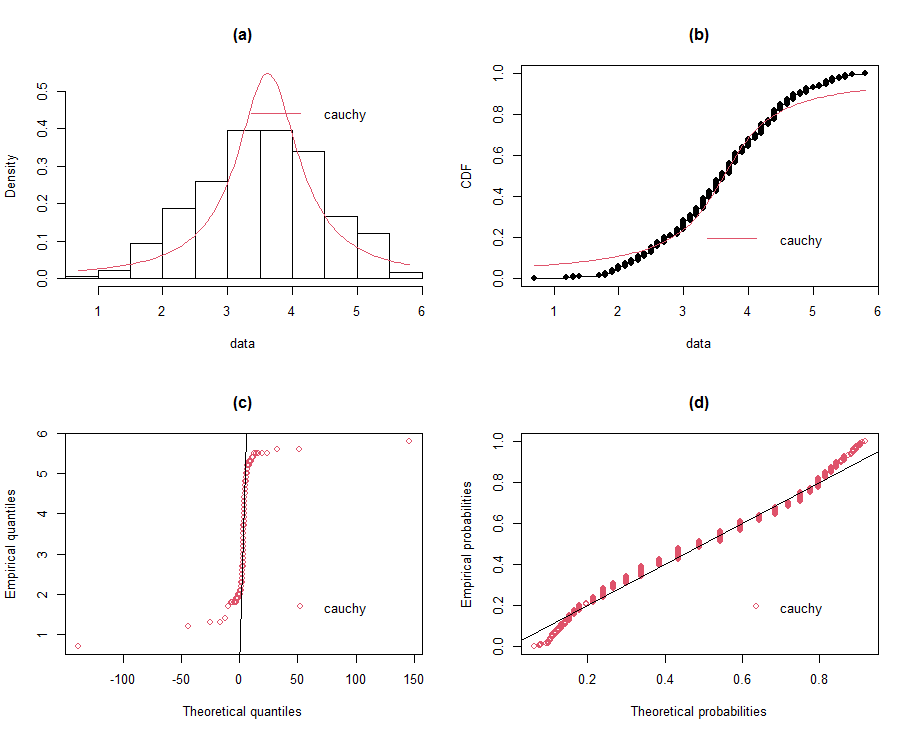 | Figure 6 (a-d). Fitted Cauchy distribution |
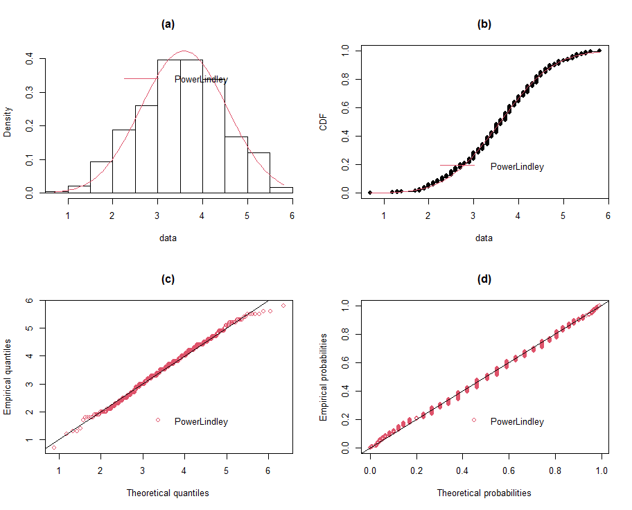 | Figure 7 (a-d). Fitted power Lindley distribution |
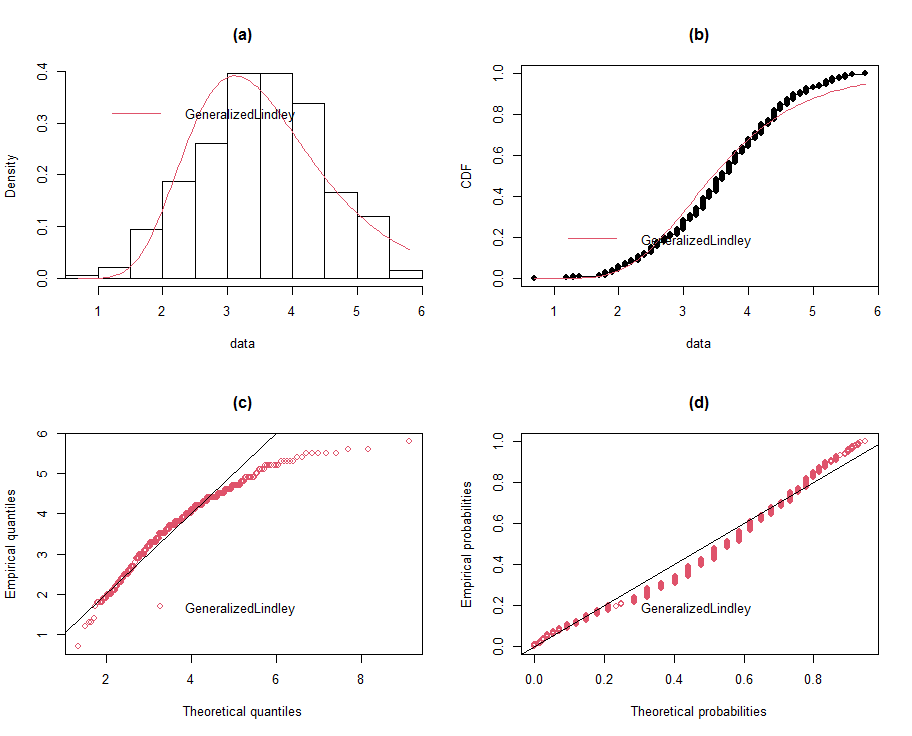 | Figure 8 (a-d). Fitted generalized Lindley distribution |
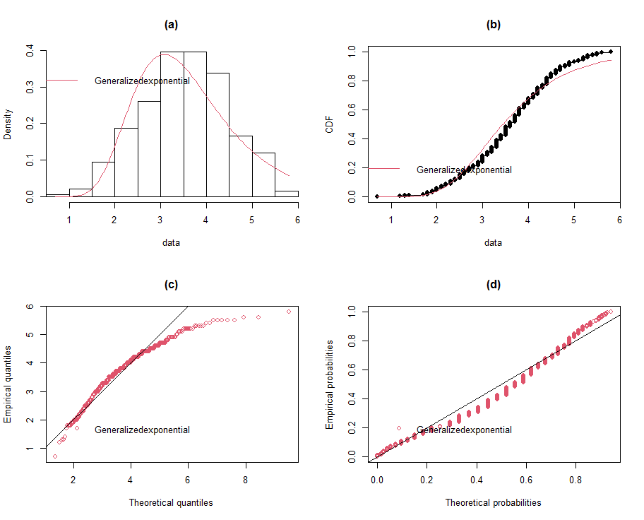 | Figure 9 (a-d). Fitted generalized exponential distribution |
 | Figure 10 (a-d). Fitted generalized Rayleigh distribution |
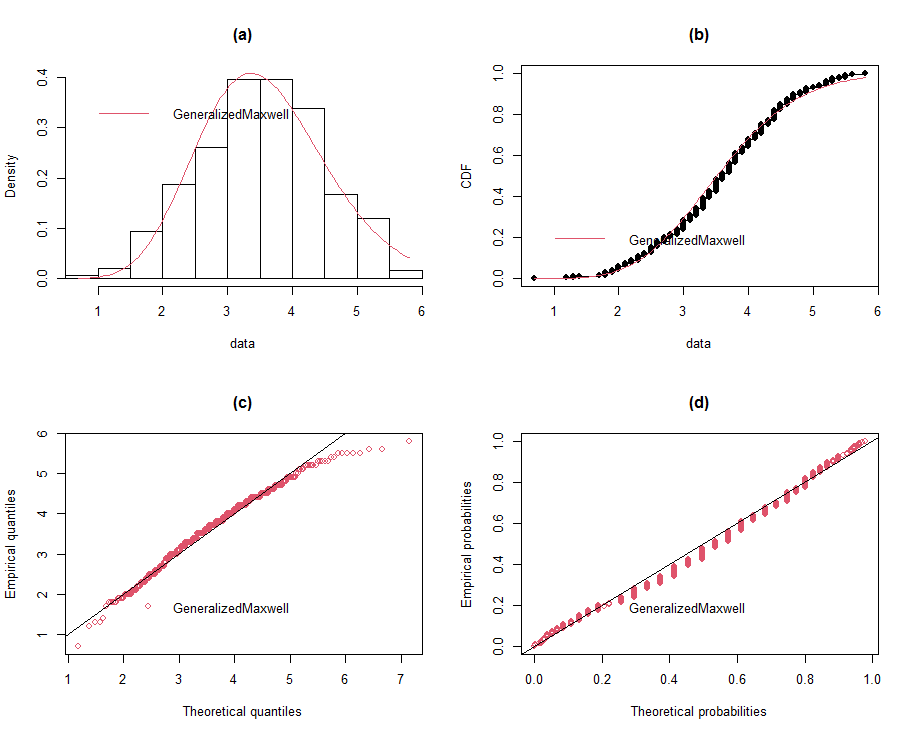 | Figure 11 (a-d). Fitted generalized Maxwell distribution |
5. Summary and Conclusions
- The modeling of wind speed observations from South-East Nigeria has been carried out in this study. Ten probability distributions were used to fit the wind speed sample from the region for the period (1987 – 2019). The ten distributions include the well-known Weibull model which is the dominant model in wind speed studies, and nine other 2-parameters distributions. The maximum likelihood method was used to estimate the parameters of all the distributions. The results obtained from the study clearly showed that the normal and power Lindley distributions proved to be a very efficient alternative to the Weibull distribution. This has spurred our suggestion that these two models should also be considered when carrying out wind speed analysis for the region. We hope that this study will beckon the attention of other researchers working within the area of wind speed modeling.
ACKNOWLEDGEMENTS
- The authors wishes to express our appreciation to TETFund for approving and releasing funds for this study through the Institution-Based Research programme for full sponsorship of this work; and sincerely thank the Management of Federal Polytechnic Nekede, Owerri, Imo State, Nigeria, for graciously approving and positively recommending this proposal.