Sahar Khairyfarag, Zohdy Mohamed Nofal, Mohamed Goda Hindawy
Department of Statistics, Mathematics and Insurance, Banha University, Egypt
Correspondence to: Sahar Khairyfarag, Department of Statistics, Mathematics and Insurance, Banha University, Egypt.
| Email: |  |
Copyright © 2022 The Author(s). Published by Scientific & Academic Publishing.
This work is licensed under the Creative Commons Attribution International License (CC BY).
http://creativecommons.org/licenses/by/4.0/

Abstract
When a parametric form for the underlying distribution is not available, the estimation of hazard quantile is of major interest. Furthermore, the hazard quantile function can be employed instead of the hazard function. This work describes a new nonparametric hazard quantile function estimator based on TL-moments approaches in detail.
Keywords:
Quantile, Hazard, Hazard quantile, TL-moments
Cite this paper: Sahar Khairyfarag, Zohdy Mohamed Nofal, Mohamed Goda Hindawy, On Nonparametric Methods for Estimating the Hazard Function with Application, International Journal of Probability and Statistics , Vol. 11 No. 1, 2022, pp. 9-18. doi: 10.5923/j.ijps.20221101.02.
1. Introduction
The statistical analysis of time-to-event data shows a main role in many of various application areas such as, industrial (reliability testing), medical (survival analysis), and demographic (migration analysis, life events research). The hazard rate is used greatly as a methodological tool in these types of usages to define the instantaneous risk of observing the event of interest over time.The L-moments and TL-moments have an appealing property that the system of moments does not have; see Hosking (1990). L-moments of any order k, for example, exist. The entire sequence of L-moments is available for heavy-tailed distributions under only a finite first moment assumption. The weaker assumption of L-moments is used to describe TL-moments, which does not require a finite first moment assumption.The estimation of the hazard function is crucial in many statistical applications, especially in the data-analytic and functional statistical methods advocated by Nair and Sanakaran 2009.
2. Quantile Function in Term of TL-Moments
In statistical analysis, the quantile function method is a valuable tool.The method of moments is widely used to measure descriptive features of a univariate distribution, but its application is limited to sufficiently light-tailed distributions; see Bera and Bilias2002. The sequence of L-moments and TL-moments, which take the form of expectations of selected linear functions of order statistics, offer an appealing alternative. is defined as:
 | (1) |
 is the population cdf. If F is an absolutely continuous with density f =
  and is one-to -one Q is differentiable on the open unite intrveral,
  And
And  is called the quantile density function (qdf). In this case
 . Differentiation on both sides give
  the function
  is called the density quantile function; see Parzen (1979), Cheng and Parzen (1997) and Cheng (2002). Thus, the density quantile function is another related quantity which obtained from the pdf,
  by substituting for x with the quantile function, as see Parzen (1979).
 | (2) |
As  and
and  for any paire of values
  it follows from the deffinition of differention that
 Hence
Hence  and, therefore, expressing all in terms of
  The two functions
  are thus reciprocals of each other. Thus, the density-quantile function can be defined in terms of quantile density function as
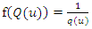 Otherwise, the quantile density function can be defined in terms of density quantile function as:
 | (3) |
3. Representation of Density Quantile Function in Terms of TL-Moments
Hosking (2007), derived the TL-moments as the coefficients in the expansion of the quantile function in the form of a weighted sum of shifted Jacobi polynomials as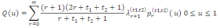 | (4) |
where  is shifted Jacobi polynomials which is given by
 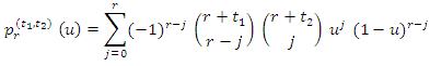 | (5) |
and, 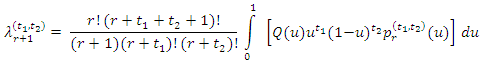 | (6) |
This is convergent in the weighted mean square with weight function  , i.e.
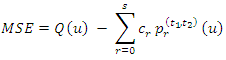 | (7) |
the remainder after stopping the sum, after s terms, satisfies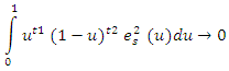 It also represents of density function in terms of TL moments by the following theoremLet X be a continuous real-valued variable such that its trimmed mean is finite, quantile function.
 density function
  And Quantile density function
  and trimmed
  than theRepresentation
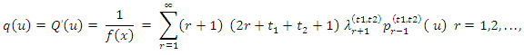 | (8) |
This is convergent in the weighted mean square with weight function  This imply that
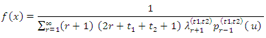 | (9) |
4. Hazard Quantile in Term of TL- Moments
Nair and Sankaran introduced hazard quantile function as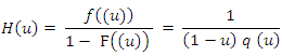 Where q(u) is the quantile density function defined by
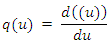 From equation (8) and (9)
 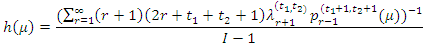 | (10) |
This is convergent in the weighted mean square with weight function  i.e.
i.e.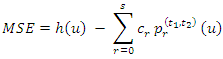 | (11) |
proof:let 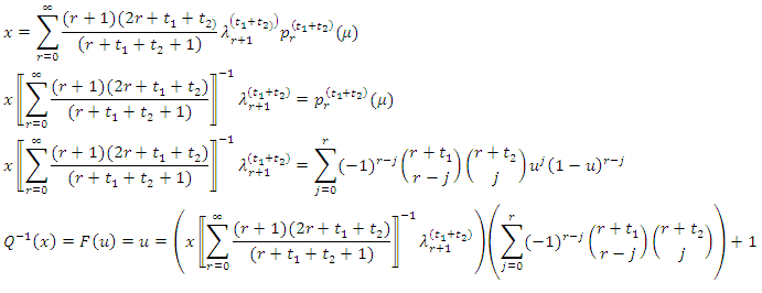
5. Estimation of the Hazard Quantile Function
From a random sample x1,x2,……………,xn of size n from the population where its corresponding order statistics is x1:n < x2:n <……………< xn:n by replacing the population TL-moments  by it sample version sample TL-moments
  From (4) we can estimate the quantile function as
 | (12) |
While, from (8) we can estimate the quantile density function 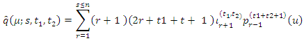 | (13) |
Thus, from (10) the hazard quantile function can be estimated as 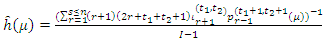 | (14) |
6. Optimal Trimming Depends on the Hazard Quantile Function
There is method for obtaining optimal trimming depends on the hazard quantile function.The error between the hazard quantile function and its TL- moments representation, in (14) can be written as 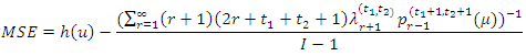 | (15) |
The optimal values of t1 and t2 can be chosen as the values which have less sum of the absolute error  Where
Where 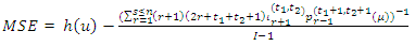 | (16) |
7. Application
We study the approximation of hazard quantile, h(u), based on TL-moments in this section, using some known distributions and real data. Using the formulas (16) and (15) that meet the two requirements in (10) and respectively (11) for different values of trimming (t1, t2) and terms (r), we compute the sum absolute error  which is given in (16).As the basis of our comparisons, we simulate 50,100, and150 observations from log normal and normal distributions. We take the hazard quantile which have
  and, in the same time, best fitting to distribution. In addition, we will compare this new approximation of the hazard quantile with the corresponding histogram and kernel density.
7.1. Lognormal Distribution
X ∼ log normal  is used to indicate that the random variable
  has the log normal distribution with parameters
  and
and  . A log normal random variable
  with parameters
  and
and  has probability density function
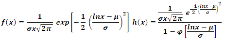
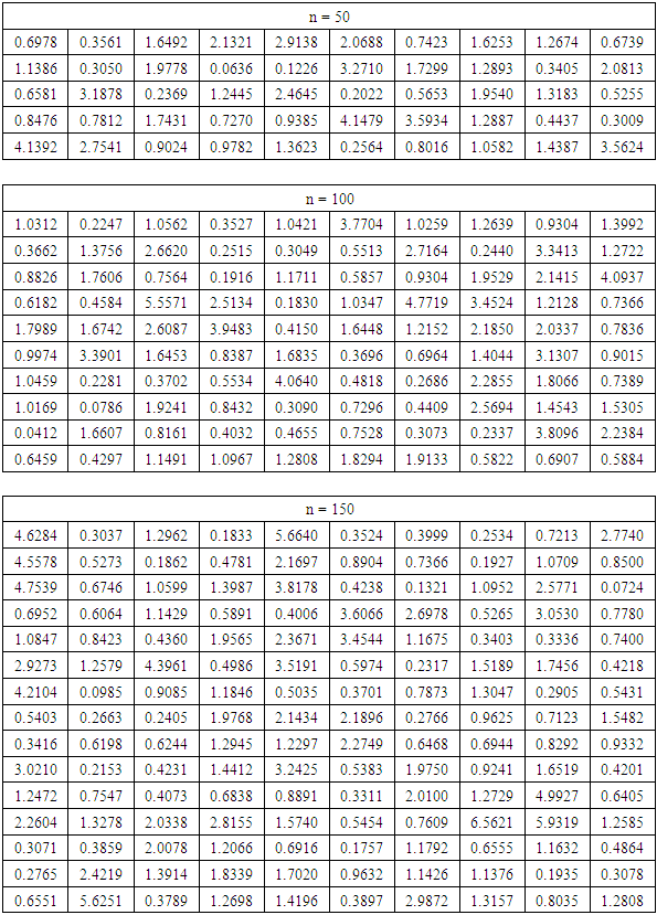
Table 1. Simulated data from lognormal distribution with µ = 0 and σ = 1 using n = 50, 100, 150
 |
| |
|
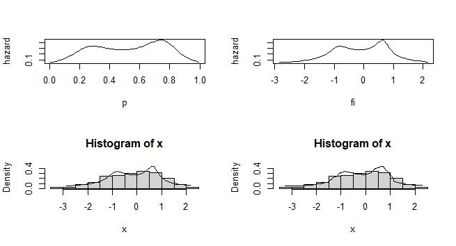
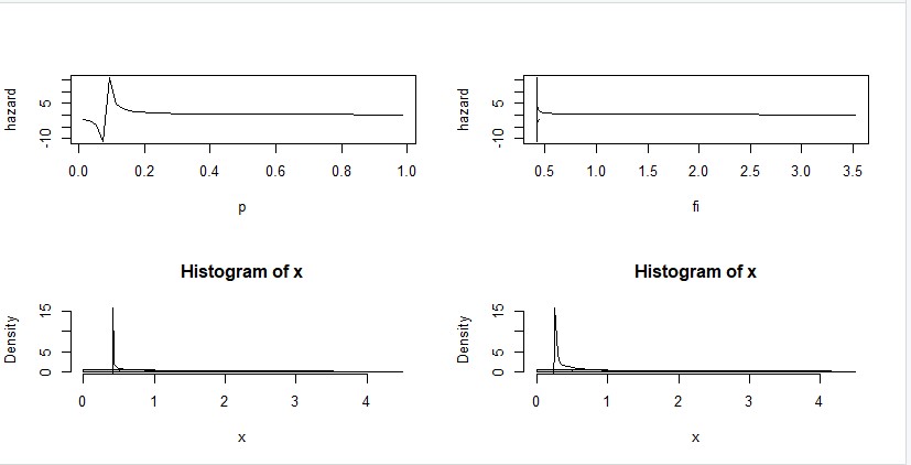 | Figure 1. Approximation of the hazard and density functions of lognormal distribution (µ = 0 and σ = 1), using terms (r=3), trimming (t1=1, t2=1) and sample size n=50 |
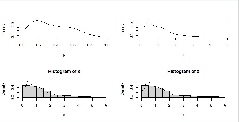 | Figure 2. Approximation of the hazard and density functions of lognormal distribution (µ = 0 and σ = 1), using terms (r=6), trimming (t1=1, t2=1) and sample size n=100 |
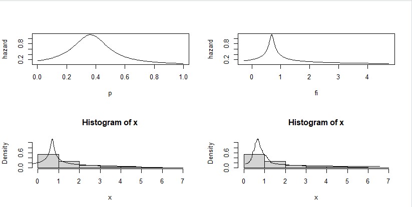 | Figure 3. Approximation of the hazard and density functions of lognormal distribution (µ = 0 and σ = 1), using terms (r=4), trimming (t1=1, t2=1) and sample size n=150 |
7.2. Normal Distribution
Normal distributions are useful in statistics and are often used in the natural and social science for real valued random variables whose distributions are not known. If X is distributed according to the normal distribution, then 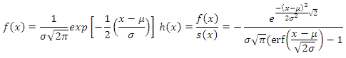
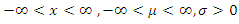
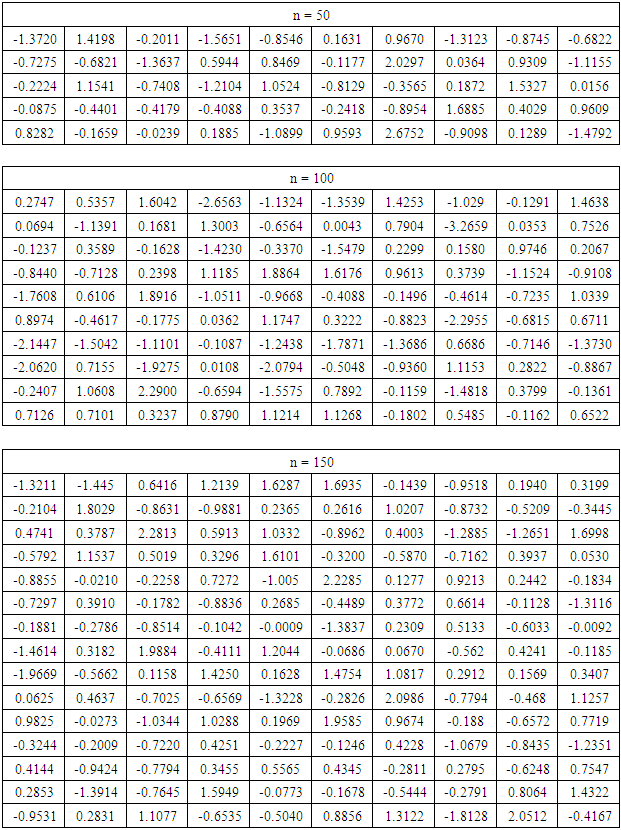
Table 2. Simulated data from normal distribution with µ = 0 and σ = 1 using n = 50, 100 and 150
 |
| |
|
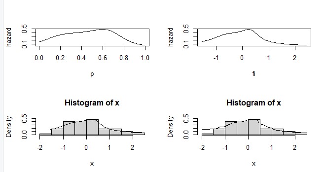
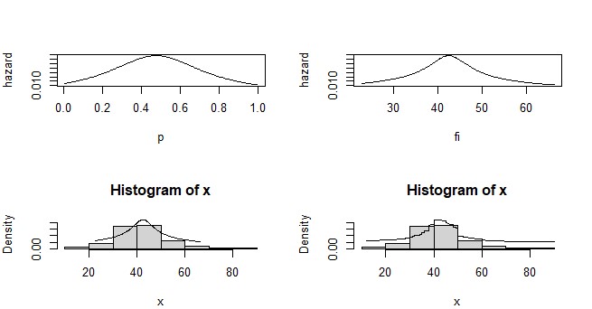
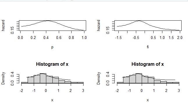 | Figure 4. Approximation of the hazard and density functions of normal distribution (µ = 0, σ = 1), using terms (r=6), trimming (t1=1, t2=0) and sample size n=50 |
 | Figure 5. Approximation of the hazard and density functions of normal distribution (µ = 0, σ = 1), using terms (r=6), trimming (t1=0, t2=0) and sample size n=100 |
 | Figure 6. Approximation of the hazard and density functions of normal distribution (µ = 0, σ = 1), using terms (r=6), trimming (t1=1, t2=1) and sample size n=150 |
7.3. Real Data
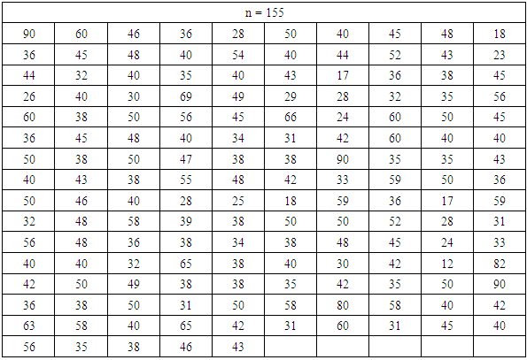
We add an approximation to the hazard quantile function for real data using the same technique of approximation to know distributions.Table 3 shows the ages of 155 patients with Stomach Tumors who were admitted to (Zagazig University Hospital, Pain Clinic, Egypt) between June and December 2020.Table 3. Data of the ages for 155 patients of Stomach Tumors taken from (June-December 2020) whose entered in (Zagazig University Hospital, Pain Clinic, Egypt)
 |
| |
|
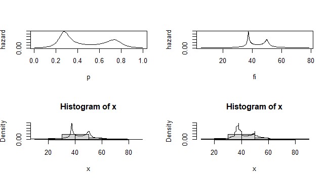
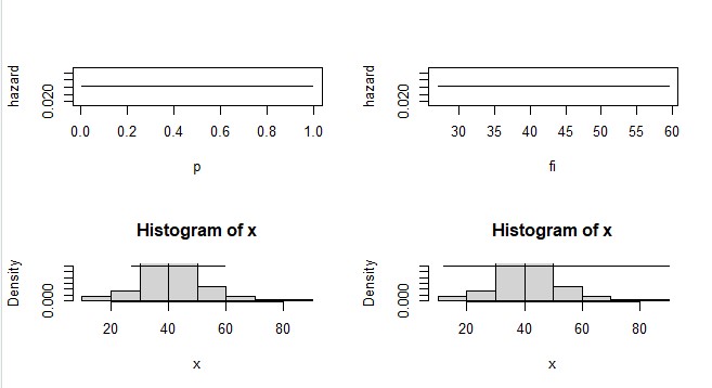 | Figure 7. Approximation of hazard quantile function of Stomach Tumors size n=155, trimming (t1=1,t2=2) and using two terms (r=2) |
 | Figure 8. Approximation of hazard quantile function of Stomach Tumors size n=155, trimming (t1=1,t2=2) and using four terms (r=4) |
 | Figure 9. Approximation of hazard quantile function of Stomach Tumors size n=155, trimming (t1=1,t2=2) and using six terms (r=6) |
8. Conclusions
The population hazard function (which indicated the approximation of hazard quantile function) is approximated using a nonparametric methodology based on the TL-moments and the orthogonal Jacobi polynomial as an approximation. This methodology has the capacity to acquire more information regarding the data's arbitrary distribution. This method is focused on reducing the sum absolute error between the population hazard quantile function and its portrayal in TL-moments.Unlike its parametric counterpart, there is no need to make any assumptions about the underlying distribution. We also used symmetric and asymmetric distributions to demonstrate the benefits of the suggested technique.The performance of the proposed estimator is tested by applications to real-life and simulated data. Also, a comparison of its performance to that of the normal estimator indicates that the lognormal estimator performs better than that of the normal estimator near the boundary.
References
| [1] | Abd-Elrazek E. M., (2015). On the use and application of trimmed L-moments. phd thesis , Benha University, Faculty of Commerce, Department of Statistics, Mathematics, and Insurance. |
| [2] | Abd-Elrazek E. M., Qandeel, A. M., and Habib, S. A. (2015). Nonparametric Estimation for Density Quantile Function Via TL-Moments. Int. J. Bus. Stat. Ana., 2, No. 1, 21-39. |
| [3] | Afshari M. and Tahmasebi S., (2014). estimation hazard of function for censoring random variable by using wavelet decomposition and evaluation of MSE. journal of data analysis and information processing 2, 1-5. |
| [4] | Akcin H., Zhao Y., Jiang Y., and Zhang X., (2018). Nonparametric Estimation of a Cumulative Hazard Function with Right Truncated Data. New frontiers of biostatistics and bioinformatics. 403-420. |
| [5] | Akcin H., Zhang X., and Zhao Y., (2018). Nonparametric Estimation of a Hazard Rate Function with Right Truncated Data. New frontiers of biostatistics and bioinformatics. 441-456. |
| [6] | BABU G. J., (1986). Estimation density quantile function, the indian journal of statistics 48, ser. A, Pt.2 142-149. |
| [7] | Elamir E. A. H. and Seheult, A. H., (2003). Trimmed L-moments. Computational Statistics Data Analysis 43, 299-314. |
| [8] | Elamir E. A. H., Kandile, A. M. and Enayat, M. A., (2009). FL-moments. Cairo University, Institute of Statistical studies and research, The Annual Conference on Statistics, Computer science and operation research, 15-30. |
| [9] | Gefeller, O., (1994). Nonparametric estimation of the hazard rate: statistical methods, examples, and software (un-) availability. In SAS Institute Inc. (ed.). SEUGI/Club BAS '94. Proceedings of the 12th SAS European Users' Group International Conference Strasbourg. (pp. 1037-1044). Heidelberg: SAS Institute. |
| [10] | Laura spierdijk., (2008). Nonparametric conditional hazard rate estimation, journal of computational statistical and data analysis 52, 2419 – 2434. |
| [11] | M. O. Mohamed. (2020). Estimation of R for geometric distribution under lower record values. Journal of Applied Research and Technology, 18(6), 368-375. |
| [12] | Nair N. U., and Sankaran, P. G., (2009). Nonparametric estimation of hazard quantile function. Journal of Nonparametric statistics, 21, 757-767. |
| [13] | Nair, N. U., and Sankaran, P. G., (2009). Quantile-based reliability analysis. Communications in Statistics - Theory and Methods, 38(2), 222–232. |
| [14] | Padgett W. J., (1988). Nonparametric estimation of density and hazard rate functions when samples are censored. In Krishnaiah, P.R. & Roo, C.R. (eds.). Handbook of Statistics, Vol. 7 (pp. 313-331). |
| [15] | Salha R.B., Elshekh H. I., and Alhoub I. M., (2014). Hazard rate function estimation using weibull kernel, journal of statistics 4, 52 – 11. |
| [16] | Salha R.B., Elshekh H. I., and Alhoub I. M., (2014). Hazard rate function estimation using Erlang kernel, journal of statistics 3, 141 – 152. |
| [17] | Salha R.B. and Rasheed A.J., (2017). A comparison study between three different Kernel estimators for the Hazard rate function. Electronic Journal of Applied Statistical Analysis. 10. NO1. |
| [18] | Salha R.B., Elshekh H.I., and Alhoub I.M., (2017). On Improvement of Hazard Rate Function Estimation Using Adaptive Kernel Estimates. IUG Journal of Natural Studies. 25. No3. |
| [19] | Sankaran P.G. and Gleeja V.L., (2007). non parametric estimation of reversed hazard rate, calcutta statistical association bulletin 59. |

 Abstract
 Reference
 Full-Text PDF
 Full-text HTML