-
Paper Information
- Paper Submission
-
Journal Information
- About This Journal
- Editorial Board
- Current Issue
- Archive
- Author Guidelines
- Contact Us
International Journal of Probability and Statistics
p-ISSN: 2168-4871 e-ISSN: 2168-4863
2022; 11(1): 1-8
doi:10.5923/j.ijps.20221101.01
Received: Dec. 16, 2021; Accepted: Jan. 12, 2022; Published: Jan. 21, 2022

Lebesgue−Chebyshev Synergism for the Bounds of Measurable Random Variables
 Abstract
 Reference
 Full-Text PDF
 Full-text HTML
Francis Egenti Nzerem, Ukamaka Cynthia Orumie
Department of Mathematics and Statistics, University of Port Harcourt, Choba, Nigeria
Correspondence to: Francis Egenti Nzerem, Department of Mathematics and Statistics, University of Port Harcourt, Choba, Nigeria.
| Email: |  |
Copyright © 2022 The Author(s). Published by Scientific & Academic Publishing.
This work is licensed under the Creative Commons Attribution International License (CC BY).
http://creativecommons.org/licenses/by/4.0/

The attainment of a near-faultless optimal estimate is always the chief goal in the application of measures. Boundedness is always an ‘essential commodity’ if optimality is desired. A function is Lebesgue integrable if theLebesgue integral does not ‘explode’; as well the existence of Chebyshev bound assures that the estimates of certain random variables or those of certain functionals, as the case may be, do not ‘explode’. The realization of the latter has the underpinning of Lebesgue measure applied on the set functions under consideration. Therefore, this work treated a veritable way of estimating the (maximal and minimal) bounds of Chebyshev-type inequalities, with the functions presupposed Lebesgue measurable.
Keywords: Lebesgue−Chebyshev, Inequalities, Bounds, Maximal function, Probability
Cite this paper: Francis Egenti Nzerem, Ukamaka Cynthia Orumie, Lebesgue−Chebyshev Synergism for the Bounds of Measurable Random Variables, International Journal of Probability and Statistics , Vol. 11 No. 1, 2022, pp. 1-8. doi: 10.5923/j.ijps.20221101.01.
Article Outline
1. Introduction
- The central limit theorem in mathematical probability theory reckons that, often, the addition of independent random variables to the original variables causes the normalized sum of such variables to tend toward a normal distribution even though they are not normally distributed. However, the central theorem affords simply an asymptotic distribution, and it requires several observations to stretch into the tails of a normal distribution. Chebyshev’s Inequality is widely used in probability theory, and; it furnishes probability bounds on wide-ranging aspects of probability distributions. The central importance of the inequality is the use in limiting the distance between the mean and a random variable, Amaresh [1]. As precious as the inequality is in doing the said work, its drawback is the inability to employ it in setting confidence intervals in estimation problems. However, the propitiation of this Chebyshev’s shortcoming is the use of concentration inequalities (see [2], [3], [4]). Besides, Roos et al. [5] provided alternative tight lower and upper bounds on the tail probability under certain conditions. Such bounds were obtained as exact solutions to semi-infinite linear programs.Chebyshev’s inequality is, fundamentally, a consequence of the measure theory, as any resulting bounding value is to be prescribed in a “measurable set”. In the light of this, Stepaniants [6] and Billingsley [7] showed that Chebyshev’s inequality can be subsumed in the theory of Lebesgue measure. Besides the qualitative use of the generic Chebyshev’s inequality in probability measures, numerous applications of Chebyshev-type inequalities furnish suitable bounds for the estimation of some class of functions. One of such celebrated functions is depicted in the abiding maximal theorem by Hardy and Littlewood [8] - a work that has engaged the attention of Flett [9], Keith [10], among numerous others found in literature. In recent times numerous Chebyshev-type inequalities are ‘crafted’ to attend to varying needs (see Teimourian and Ghazanfari [11], Nisar et al. [12])).Another salient class of inequality is the type that is obtainable from the Chebyshev functionals of functions of bounded variation. While numerous identities that relate to the Chebyshev functional were considered by Mitrinovi ́c et al. [13,14], the quest for the bounds for the functional was done by Cerone [15,16] and Dragomir [17].This work supplied the combined outcome of (Lebesgue) measure theory and Chebyshev’s inequality in furnishing the method of obtaining estimates (bounds) of functions and Chebyshev-type functionals. The linear combinations of independent random variables, their control, and the maximal averages over some parameters are desired for purposes of empirical risk minimization. In effect, this line of study is quite graceful, for purposes of optimization.
2. Preliminaries
- Some basic tools for the development of the content of this paper are supplied in this section.
2.1. The Measure Space
- Definition 1. Let
 be a measurable space. A set function μ is a measure on the space if:(i)
  ;(ii)
;(ii)  0;(iii) Given a sequence of disjoint A1, A2, . . . of
  -sets, and if
  then
then 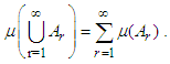 | (1) |
 is called a measure space.
 2.1.1. Probability Space
- Definition 2. Let (Ω, F) and (Ω′, F′) be two measurable spaces. The function X : Ω→S is measurable a function and
 | (2) |
 and F′ is the Borel σ-algebra.If Ω is any state space that is not endowed with σ-algebra, and X : Ω→Ω′ is a function that has value in a measurable space (Ω′, F′), then the smallest σ-algebra for which X is a measurable function is
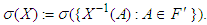 | (3) |
 is a probability space, in which:(i) Ω denotes the sample space describing a non-empty set of all possible outcomes of some model being performed.(ii) F denotes an σ-algebra on the sample space (Ω ∈F). (iii)
  is a probability measure if it as well satisfies the countably additive property specified in 2.1 (iii).Probability measures has been largely used in optimization problems as seen in Saito and Takahashi [18] and Yu [19].If X1, X2,… is a sequence of real-valued random variables defined on
  , then the supremum
 is measurable (see Lowther [20]).
2.2. Excerpts from Lebesgue Integral
- Let
 be a random variable. It has a Gaussian distribution if it has a Lebesgue measurable density p on R such that
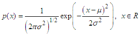 where
where  and
and  are the mean and variance of X.Let
  be a measure space:(i) If
  is an S-summable function, and SP is an S-partition B1, B2,…, Bm of X, then the lower Lebesgue sum L (f , SP) is defined by
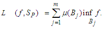 (ii) If
  and
and  is the characteristic function of D, we get (see Axler [21])
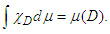 (iii) If
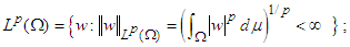
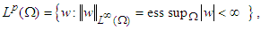
 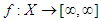 is S-summable, then the Lebesgue space
  reads,
 is an
is an  measurable function from
  to
to  and
and 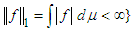 (iv) Lemma 1. If
  , then (Markov’s inequality)
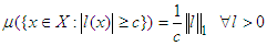 | (4) |
 | (5) |
 .
.2.3. Chebyshev’s Inequality from Lebesgue Integral
- The generic (probability) statement of Chebyshev’s Inequality reads:Theorem 1. (Chebyshev’s Inequality). Let X : Ω→R be a random variable on a probability space (Ω, F, P). Suppose X has a finite expected value m and finite nonzero variance σ2. Then, for any real number k > 0
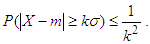 | (6) |
 | (7) |
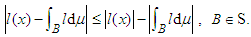 Let
Let  be the characteristic function of B. Then,
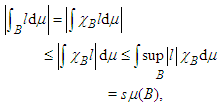 | (8) |
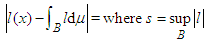 . The above shows that the integral measure
  in (7) encodes the mean value. Therefore,
  ;
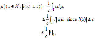
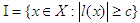
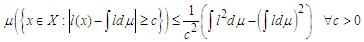
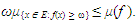
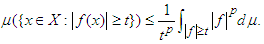
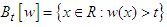
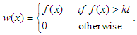
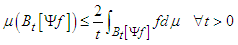
;  , we recognize the integral in the rightmost expression of (7) as equal to Var(X) = σ2. If P is the probability measure, one finds that the inequality (6) is equivalent to the inequality (7). Under some condition(s), the tail estimate of a given measurable function may be obtained using Chebyshev’s inequality. Let f be a non-negative measurable function. Define a set {x ∈ E: f(x) ≥ ω ≥ 0}. The property
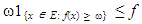 | (9) |
 | (10) |
 | (11) |
 | (12) |
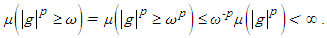
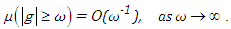
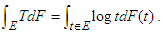
 In general, if g is an extended real-valued measurable function, nonnegative and nondecreasing, with g(t) ≠ 0 then:
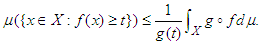 Chebyshev’s inequality may be expressed in the sense of Lebesgue integration (see Stepaniants [5]) in the theorem that follows: Theorem 3. (Generalized Chebyshev’s Inequality). Let (Y, σ, μ) be a measure space and let f be a real-valued measurable function defined on Y. Suppose μ is the Lebesgue measure and let h be a non-negative and non-decreasing real-valued measurable function on the range of f. Then, for any positive real number n and 0 < t < ∞,
 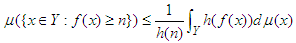 | (13) |
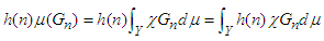
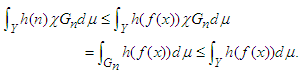
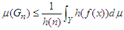
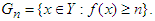 Denote the characteristic function of the set Gn by χGn. By the theorem, h is non-decreasing and it is non-negative on the range of f, therefore
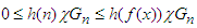 | (14) |
 | (15) |
 | (16) |
 | (17) |
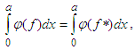
2.4. Equi-measurable Functions
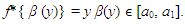
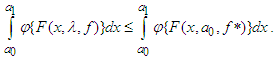
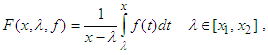
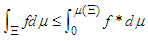
- So far, the emphasis had been on non-decreasing functions. What happens if a function is decreasing in an interval? The relationship between the above two types of functions is well articulated in the seminal and yet abiding work by Hardy and Littlewood [8].Assume that f(x) is a positive, bounded, and measurable in (a0, a1); let β(y) be a measure such that f(x) ≥ y, therefore β(y) is a decreasing function of y which vanishes for sufficiently large y. The function f*(x) is defined for x ϵ [a0, a1] by
 | (18) |
 | (19) |
 | (20) |
 | (21) |
 | (22) |
 | (23) |
 | (24) |
 | (25) |
 | (26) |
 .
.3. Estimation of Bounds
- The estimation of the bounds of measurable functions is of much importance in applicable phenomena. Inequality measures contribute much to near guileless estimates. Extensive energies that have so far been expended on the theory of maximal inequalities for several decades have produced a sumptuous result. As expected, such inequalities must be rigged in the Lebesgue
 function space if the bounds are to be sought. This section is devoted to inequality bounds that are consequences of Chebyshev’s inequality and with the underpinning of
  measures.
3.1. Bounds in Function  Spaces
3.1.1. Probability Bound
- Many a time the linear combinations of independent random variables, their control, and the maximal averages over some parameters are desired for purposes of empirical risk minimization. Let P be a probability distribution over some set X. An ε-net for a class
 of subsets X is any subset
  such that for any qϵ H
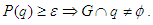 .The subset G approximates the probability distribution. An ε-approximation for class H is such that [23]
 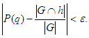 The following argument derives from [24].Let X1,..., Xn be n independent and random variables such that E[Xi] = μ and var(Xi) ≤ σ2 . Let δ ∈ (0, 1) and assume that n can be factored into n = K·W where W = 8 log(1/δ) is a positive integer. For w = 1, ..., W, let
  denote the average over the w-th group of k variables. Then, this average takes the form
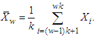 For any w = 1,...,W, it can be shown [24] that
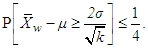 | (27) |
 as the median of {X1,..., XW}. Then
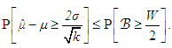 where B ∼ Bin(W, 1/4). Evidently,
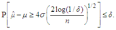 | (28) |
 | (29) |
 | (30) |
 Consider the L2 ball. Let
  be fixed and let ε > 0. A set G is called an ε-net of
  with respect to a distance d(·, ·) on Rd, if
  and for any
  there exists x ∈G such that d(x, z) ≤ ε. The unit L2 ball of Rd is the set of vectors u that have Euclidean norm |u|2 at most 1, usually defined by
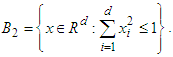 The upper bound on the magnitude of the smallest ε-net of
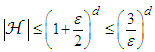
  is given below.Lemma 4. [24] Let ε ∈ (0, 1). Then the unit Euclidean ball
  has an ε-net
  with respect to the Euclidean distance of cardinality
  Proof. Going by [24], construct an iteration of the ε-net. Choose x1 = 0. For a given i ≥ 2, let xi be any
  such that |x−xj|2 > ε for all j < i. If there is no such x, stop the process. Thus, an ε-net is generated. Then, the size of the ε-net has to be controlled.The Euclidean balls centred at
  and with radius ε/2 are disjoint as |x−y|2 > ε for all
  Besides,
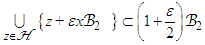 | (31) |
 . Thus, measuring volumes, one finds
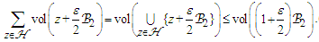 | (32) |
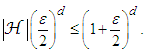 | (33) |
 | (34) |
 | (35) |
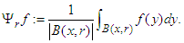
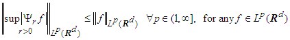
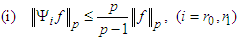
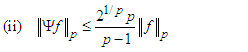
 the operators ψr are contractions for which Young’s inequality
 | (36) |
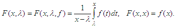
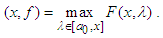
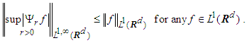
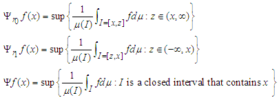
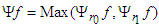
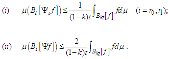
 -measurable function, f, the maximal function is of the form
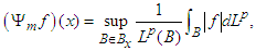 | (37) |

 | (38) |
 | (39a) |
 | (39b) |
 | (40) |
 | (41) |
 | (42) |
 | (43) |
 | (44) |
 and we have
 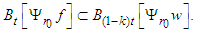 Since the equality
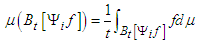 | (45) |
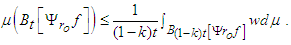 | (46) |
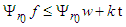
 since w = 0 there. Thus
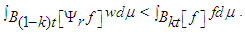 | (47) |
 | (48) |
 | (49a) |
 | (49b) |
3.2. Chebyshev Functional
- The bounding of the Chebyshev functional has extensive applicability in probability problems and the bounding of special functions in applied mathematics. Some theories and identities that relate to the Chebyshev functional are treated in Mitrinovi ́c et al. [13,14] while Fink [25] looked at an applicable aspect of such inequalities. Elegant and enduring work in the quest to bound the Chebyshev functional was done by Cerone [15].As usual, let f, g: [a,b]→
 be two measurable functions. The weighted Chebyshev functional W(f, g) is defined by
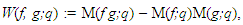 | (50) |
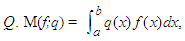 where
where 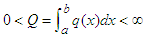 and the above integral is assumed to exist. The following equivalences hold [22],
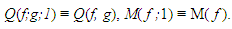 | (51) |
 are two equi-monotonic functions, then
 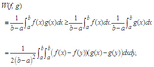 | (52) |
 | (53) |
 be a measure space, with μ as a countably additive and positive measure on σ with values in R ∪ {∞}. Given a μ-measurable function
  , with v(x) ≥ 0 for μ, a.e. x ∈ X, define a Lebesgue space
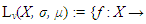
 , f is μ-measurable and
 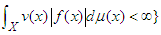 . Assume
  If f, g: X →
  are μ-measurable functions and f, g, f g ∈ Lv (X, σ, μ), then the Chebyshev functional that admits v(x) may be written as
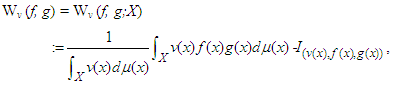 | (54) |
 In Cerone [15], remarkable work was done in using the above to furnish some bounds. As well, the bounds for the modulus of complex Chebyshev functionals engaged the attention of Dragomir [17]. In Grüss [26], the Chebyshev functional was evaluated as
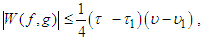 | (55) |
 are real numbers such that
 The constant ¼ is assumed sharp, as there would be no smaller number in its stead. The proof of this inequality is available in Mitrinovi ́c et al. [13].
3.3. Bound for the Generalized Prime Numbers
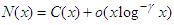
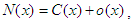
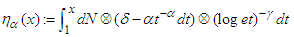
- Beurling [27] conducted an extensive and enduring study on the asymptotic distribution of prime numbers. The distribution function N(x) for the generalized prime numbers satisfies the inequality
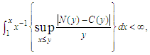 | (56) |
 | (57) |
 | (58) |
 | (59) |
 | (60) |
 | (61) |
 | (62) |
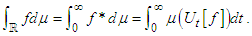
 | (63) |
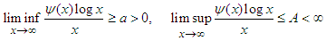
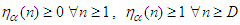
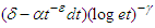 , where δ encodes the Dirac measure at 1, dt is the Borel-Lebesgue measure on [1,∞) and α is a positive number. Then we state, without proof, the following lemma whose proof furnishes Chebyshev’s upper and lower bounds.Lemma 6. Suppose that (36) holds with C > 0 and γ >1. Then there exists a positive number α depending on N(x) that satisfies the conditions: (i)
 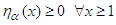 (ii)
(ii) 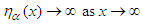 The proof of the above lemma is available in Diamond [31]. As a result, the upper bound is satisfied by
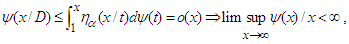 | (64) |
 . The lower bound is satisfied by
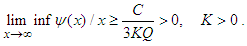 | (65) |
4. Summary and Conclusions
- The achievement of a near-flawless optimal estimate is always a desirable end. Boundedness is always a sine qua non to the achievement optimality. The linear combinations of independent random variables, their control, and the maximal averages over some parameters are desired for purposes of empirical risk minimization. This work supplied the (Lebesgue) measure theory and Chebyshev’s inequality synergism in providing the method of obtaining estimates (bounds) of functions and Chebyshev-type functionals which may be applicable in such risk minimizations.Chebyshev’s inequality in the main is a consequence of the measure theory, as any resulting bounding value is embedded in a “measurable set”. It was shown in this work that Chebyshev’s inequality and Chebyshev-type inequalities can be subsumed in the theory of (Lebesgue) measures. Besides the qualitative use of the generic Chebyshev’s inequality in probability measures, numerous applications of Chebyshev-type inequalities provide appropriate bounds for the estimation of some class of functions. This reasoning calls for an in-depth study of measure theory as it acts as a catalyst to the resolution of optimization problems.
ACKNOWLEDGEMENTS
- The authors are grateful to the reviewers for their useful suggestions that led to the revision of this work.