Abdul-Hadi N. Ahmed 1, Zohdy M. Nofal 2, Hager N. Ahmed 2
1Department of Mathematical Statistics, Faculty of Graduate Studies for Statistical Research, Cairo University, Giza, Egypt
2Department of Statistics, Mathematics and Insurance Benha University, Benha, Egypt
Correspondence to: Hager N. Ahmed , Department of Statistics, Mathematics and Insurance Benha University, Benha, Egypt.
| Email: |  |
Copyright © 2021 The Author(s). Published by Scientific & Academic Publishing.
This work is licensed under the Creative Commons Attribution International License (CC BY).
http://creativecommons.org/licenses/by/4.0/

Abstract
In this thesis, We propose and study new compounding families, the truncated natural discrete Lindley with three distributions severally (Exponential distribution, Weibull distribution and Lomax distribution) this approach generates new distributions that extend well-known families of distributions. At the same time, they offer more flexibility for modeling lifetime data. The structural properties of the new distributions are investigated. These include the compounding representation of the distribution, reliability analysis and statistical measures. Expressions for Lorenz and Bonferroni curves and Renyi entropy as a measure for uncertainty reduction are derived.. The maximum likelihood method is used to estimate the model parameters. Two real-life data applications are proposed to illustrate the importance of the new families.
Keywords:
Exponential distribution, Weibull distribution, Lomax distribution, Lindley distribution, Reliability analysis, Moment generating function, Order statistics and Quantile, Maximum likelihood estimation
Cite this paper: Abdul-Hadi N. Ahmed , Zohdy M. Nofal , Hager N. Ahmed , New Compounded Family of Distributions, with Applications, International Journal of Probability and Statistics , Vol. 10 No. 3, 2021, pp. 74-93. doi: 10.5923/j.ijps.20211003.02.
1. Introduction
In statistical literature, we always assume that every real phenomenon can be modeled by some lifetime distributions. Modeling and analyzing lifetime data are important aspects of statistical research in many applied sciences such as engineering, medicine, economics and so on. Various recent probability distributions discussed modeling of such data by compounding the well-known lifetime distributions such as exponential, Weibull, generalized exponential, exponentiated Weibull and etc. with some discrete distributions such as zero-truncated binomial, geometric, Poisson, logarithmic and the power series distributions in general. The compounding approach gives new distributions that extend well-known families of distributions. At the same time, they offer more flexibility for modeling lifetime data. The flexibility of such compound distributions comes in terms of one or more failure rate shapes that may be decreasing, increasing, bathtub shaped or unimodal shaped. The relevance of mixtures in the analysis and improvements of coherent systems has been pinpointed in various investigations (see, for instance, Navarro et al. (2008) On the application and extension of system signatures in engineering reliability, where comparisons of coherent systems and mixed coherent systems are considered, Samaniego et al. (2007), Dynamic signatures and their use in comparing the reliability of new and used systems, where similar analysis are performed in a dynamic reliability setting, or Dugas et al. (2007), On optimal system designs in reliability-economics frameworks, who showed that solutions to certain optimization problems in reliability turn out to be mixed rather than coherent systems). We propose and study new compounding families will be named the complementary exponential truncated natural discrete Lindley distribution (CETNDL), the complementary Weibull truncated natural discrete Lindley distribution (CWTNDL) and the complementary Lomax truncated natural discrete Lindley distribution (CLTNDL), this approach generates new distributions that extend well-known families of distributions. At the same time, they offer more flexibility for modeling lifetime data. Adamidis and Loukas (1998) introduced the basic concept of these models. The basic idea of introducing compound models or families is that a lifetime of a system with N (discrete random variable) components and the positive continuous random variable, say Xi (the lifetime of the ith component), can be denoted by the non-negative random variable 
 (the minimum of an unknown number of any continuous random variables) or
  (the maximum of an unknown number of any continuous random variables), based on whether the components are in series or in parallel structure.If we define
  with cdf
  and N is a truncated discrete random variable with probability mass function
  the following steps explain how can we get the compounding of probability distribution.Step (1) obtain the conditional cdf of
  as
as where
where  is the survival function.Step (2) obtain the joint cumulative distribution function as
  Step (3) The marginal cumulative distribution of
  for the compounding distribution is given by
  If we define =
  , the following steps explain how can we get the Compounding of probability distribution Step (1) Obtain the conditional cdf of
  as
as Step (2) obtain the joint cumulative distribution function as
  The marginal cumulative distribution of
  for the compounding distribution is given by
  The rest of paper is organized as follows: Section 2 introduces the definition of the probability density function (pdf) of the (CETNDL), (CWTNDL), (CLTNDL) distributions including its cumulative distribution function (cdf) and the sub-models of the new suggested model. The reliability analysis including the survival function, the hazard (or failure) rate function, the reversed hazard rate function, the cumulative hazard rate function, and the mean residual lifetime is explored in Section 3. The statistical properties of the new distribution such as the moments, the moment generating function, and the distribution of order statistics are investigated in Section 4, with a proposed algorithm for generating random data from the new distribution in this section. Section 5 introduces Lorenz and Bonferroni curves and Renyi entropy as measures of inequality and uncertainty, respectively. Section 6 discusses the estimation of parameters by using maximum likelihood estimation. Finally, Section 7 provides an application for modeling real data sets to illustrate the performance of the new distribution.
2. Generalization and Related Sub-Models
In this section, we introduce the pdf and the cdf of the three new general compounding families and then the special cases of all distributions.
2.1. Generalization
the series systemLet  be iid from
 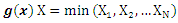 and
and  and N are independent.1. The conditional cdf of X|N is given by
 Now the joint cdf is
  This would allow us to reduce the
  is given by
  If N follows a truncated natural discrete Lindley, then
  The Cumulative distribution function (cdf) of X is given by
 We break the above sum into several components, as followsTo simplify, let
 and
and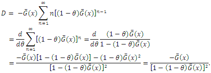 Summing up, one gets
 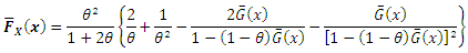 Or
Or 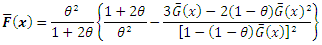 it follows that
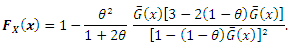 | (1) |
The associated pdf can be obtained as
 | (2) |
Next, specific well known distributions further explored.
2.1.1. N~ Complementary Exponintial Truncated Natural Discrete Lindley Distribution
Where  Then the pdf of
  for the compounding (CETNDL) distribution can be written as
 | (3) |
The compounding (CETNDL) class of distributions is defined by the marginal cumulative distribution function of  is given by
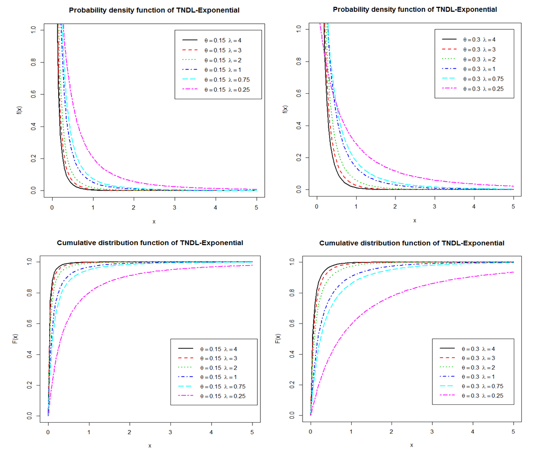 | Figure 1. Increasing, Decreasing, Constant, Bathtub and Upside-Down Shapes for cdf, pdf of CETNDL distribution, and for different values |
 | (4) |
2.1.2. N~ Complementary Weibull Truncated Natural Discrete Lindley Distribution
Every  in exp. distribution can be replaced by
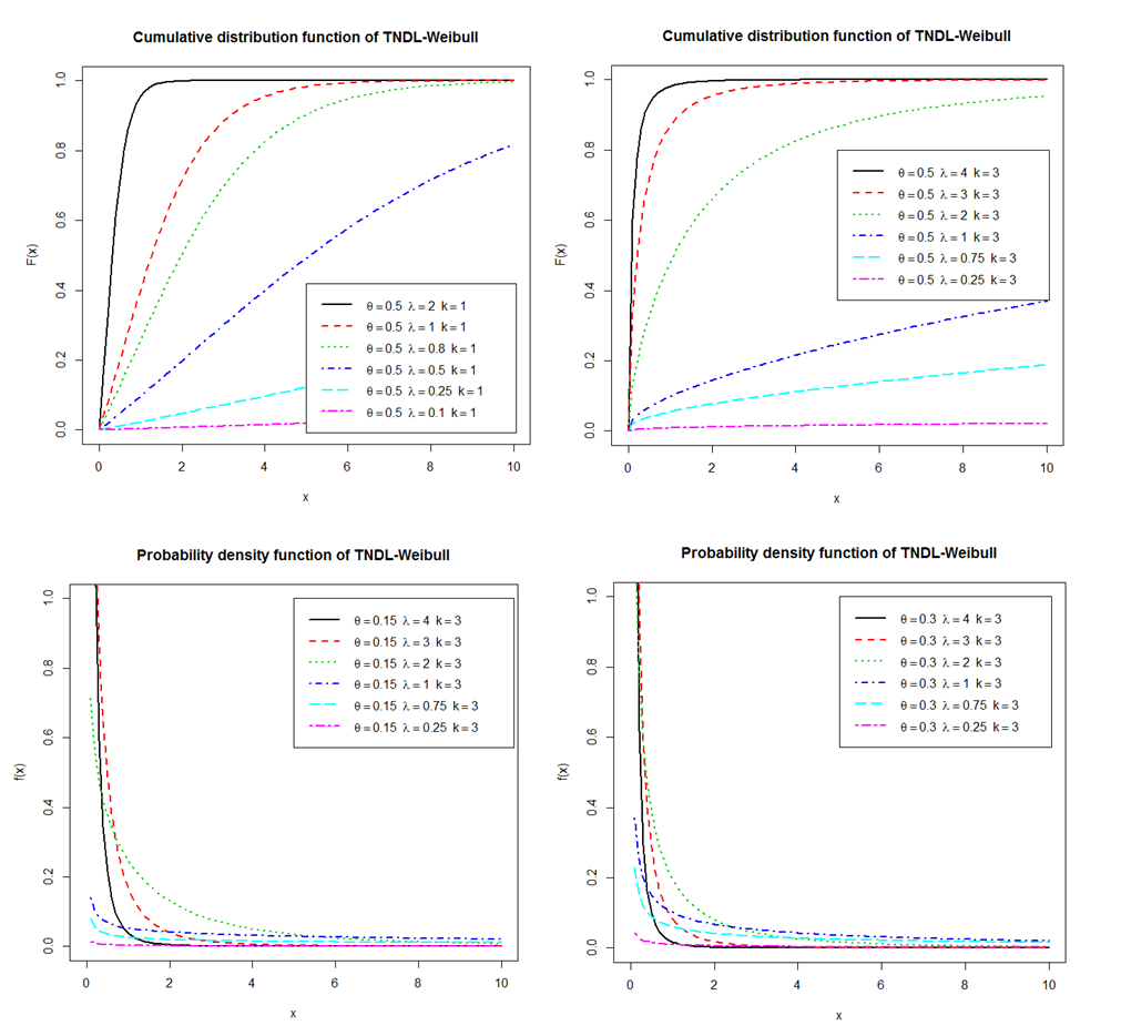 | Figure 2. Increasing, Decreasing, Constant, Bathtub and Upside-Down Shapes for cdf, pdf of CWTNDL distribution,and for different values |
Then the pdf of  for the compounding (CWTNDL) distribution can be written as
 | (5) |
the compounding (CWTNDL) class of distributions is defined by the marginal cumulative distribution function of  is given by
 | (6) |
2.1.3. N~ Complementary Lomax Truncated Natural Discrete Lindley Distribution
where  and
and  Then the pdf of
  for the compounding (CLTNDL) distribution can be written as
 | (7) |
the compounding (CLTNDL) class of distributions is defined by the marginal cumulative distribution function of  is given by
 | (8) |
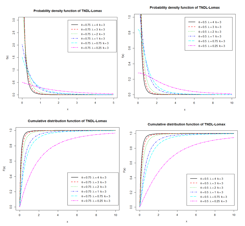 | Figure 3. Increasing, Decreasing, Constant, Bathtub and Upside-Down Shapes for cdf, pdf of CLTNDL distribution,and for different values |
3. Reliability Analysis
The time for an event to take place in an individual is called a survival time. Examples include the time that an individual survives after being diagnosed with a terminal illness or the time that an electronic component functions before failing. Two important functions for describing survival data are the survival function, the hazard function, The Reversed Hazard Rate Function, The Cumulative Hazard Rate Function, The Mean Residual Lifetime.
3.1. Survival Functions
The survival function is the probability that an observation survives longer than  that is
 Because
  is a probability, it is positive and ranges from 0 to 1. It is defined as
  and as
  approaches to
  approaches to 0. (See Lee (1992), Therefore,
3.1.1. The Survival Probability for the CETNDL Distribution is Given by
 | (9) |
3.1.2. The Survival Probability for the CWTNDL Distribution is Given by
 | (10) |
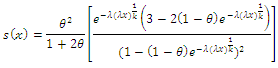
3.1.3. The Survival Probability for the CLTNDL Distribution is Given by
 | (11) |
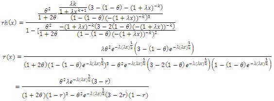
3.2. Hazard Rate Function
Nelson, (1982) defined the hazard rate is the rate of death/failure at an instant  given that the individual survives up to time t. It measures how likely an observation is to fail as a function of the age of the observation. This function is also called the instantaneous failure rate or the force of mortality. It is defined as
 where
where  is the probability density function of
  therefor
3.2.1. The Hazard Rate Function for the CETNDL Distribution is Given by
 | (12) |
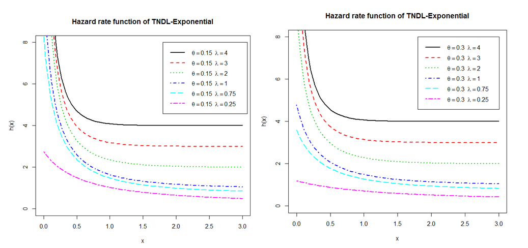 | Figure 4. Increasing, Decreasing, Constant, Bathtub and Upside-Down Shapes for the Hazad Rate Function of the CETNDL |
3.2.2. The Hazard Rate Function for the CWTNDL Distribution is Given by
 | (13) |
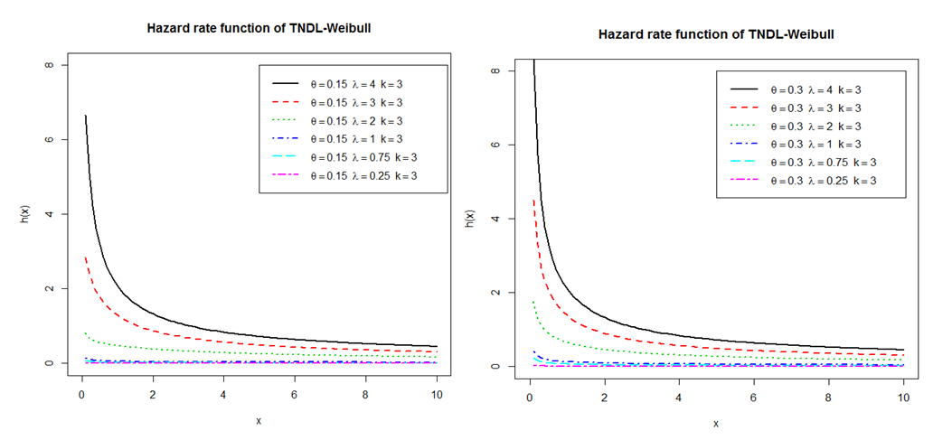 | Figure 5. Increasing, Decreasing, Constnt, Bathtub and Upside-Down Shapes for The Hazad Rate Function of the CWTNDL |
3.2.3. The Hazard Rate Function for the CLTNDL Distribution is Given by
 | (14) |
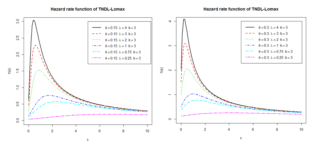 | Figure 6. Increasing, Decreasing, Constant, Bathtub and Upside-Down Shapes for The Hazad Rate Function of the CLTNDL |
3.3. The Reversed Hazard Rate Function
The reversed (reverse) hazard rate, also named retro hazard, was first mentioned by the name ‘dual of the hazard rate’ in BARLOW et al. (1963). The name ‘reversed hazard rate’ was first used by LAGAKOS et al. (1988). 6 It extends the concept of hazard rate to a reverse time direction and is defined as: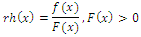
3.3.1. The Reversed Hazard Rate Function for the CETNDL Distribution is Given by
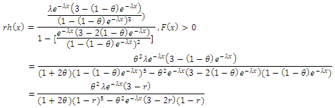 | (15) |
3.3.2. The Reversed Hazard Rate Function for the CWTNDL Distribution is Given by
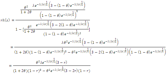 | (16) |
3.3.3. The Reversed Hazard Rate Function for the CLTNDL Distribution is Given by
 | (17) |
3.4. The Cumulative Hazard Rate or Integrated Hazard Rate CHR is Defined as
3.4.1. The Cumulative Hazard Rate Function of the CETNDL Distribution is Given by
3.4.2. The Cumulative Hazard Rate Function of the CWTNDL Distribution is Given by
3.4.3. The Cumulative Hazard Rate Function of the CLTNDL Distribution is Given by
 where
where  is the total number of failure or deaths over an interval of time, and
  is a non-decreasing function of satisfying.
4. Statistical Properties
This section investigates the statistical properties of the (CETNDL), (CWTNDL) and (CLTNDL) distributions
4.1. Distribution of Order Statistics
4.1.1. Distribution of Order Statistics for (CETNDL)
Let  be a simple random sample of size
  from CETNDL with cumulative distribution function
  and probability density function
  given by (1.1) and (1.2) respectively. Let
 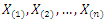 denote the order statistics obtained from this sample. The probability density function and the cumulative distribution function of the
  order statistic, say
  are given by:
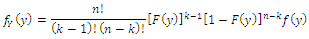 thus
thus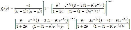 and
and
4.1.2. Distribution of Order Statistics for (CWTNDL)
Let  be a simple random sample of size
  from CWTNDL with cumulative distribution function
  and probability density function
  given by (1.1) and (1.2) respectively. Let
  denote the order statistics obtained from this sample. The probability density function and the cumulative distribution function of the
  order statistic, say
  are given by:
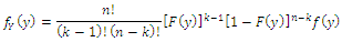 thus
thus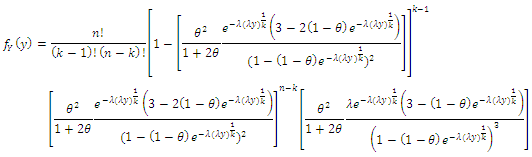 and
and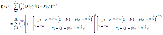
4.1.3. Distribution of Order Statistics for (CLTNDL)
Let  be a simple random sample of size
  from CLTNDL with cumulative distribution function
  and probability density function
  given by (1.1) and (1.2) respectively. Let
 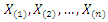 denote the order statistics obtained from this sample. The probability density function and the cumulative distribution function of the
  order statistic, say
  are given by:
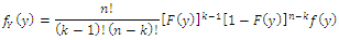 thus
thus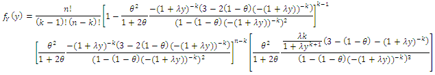 and
and
4.2. The Quantile Function
4.2.1. The Quantile Function of (CETNDL) Distribution
The quantile function  is given by:
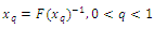 Substitute from (1.2), the quantile function is
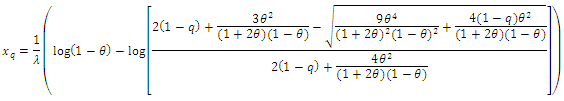 In particular when
  the median can be defined as:
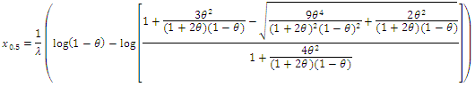
4.2.2. The Quantile Function of (CWTNDL) Distribution
The quantile function  is given by:
 Substitute from (1.2), the quantile function is
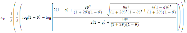 In particular when
  the median can be defined as:
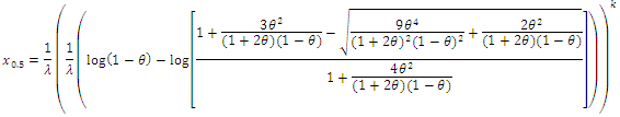
4.2.3. The Quantile Function of (CLTNDL) Distribution
The quantile function  is given by:
 the quantile function is
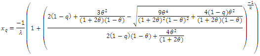 In particular when
  the median can be defined as:
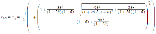
4.3. The  Non-Central Moment
4.3.1. The  Non-Central Moment for (CETNDL) Distribution
The  non-central moment is given by:
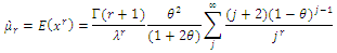
4.3.2. The  Non-Central Moment for (CWTNDL) Distribution
The  non-central moment is given by:
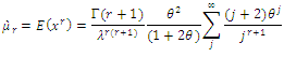
4.3.3. The  Non-Central Moment for (CLTNDL) Distribution
The  non-central moment is given by:
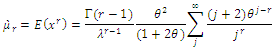
4.4. The Moment Generating Function
4.4.1. The Following Theorem Gives the Moment Generating Function (mgf) of (CETNDL) Distribution 
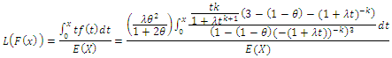
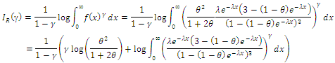
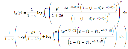
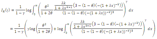
5. Measures of Inequality and Uncertainty
In this section Lorenz and Bonferroni curves are introduced as measures of inequality. Also, Renyi entropy will be mentioned as an important measure of uncertainty.
5.1. Lorenz and Bonferroni Curves
5.1.1. Lorenz and Bonferroni Curves for (CETNDL) can be Obtained as Follows
A. Lorenz curve can be obtained by B. Bonferroni curve can be obtained by
5.1.2. Lorenz and Bonferroni Curves for (CWTNDL) can be Obtained as Follows
A. Lorenz curve can be obtained by B. Bonferroni curve can be obtained by
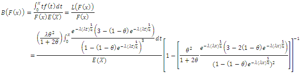
5.1.3. Lorenz and Bonferroni Curves for (CLTNDL) can be Obtained as Follows
 Bonferroni curve can be obtained by
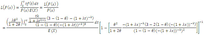
5.2. Renyi Entropy
According to Meeker and Escobar (1998) the entropy of random variable  with density function
  is a measure of uncertainty or randomness of a system. One of the popular entropy measures is Rényi entropy which is defined by
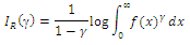
5.2.1. Rényi Entropy for (CETNDL) is Obtained as Follows
5.2.2. Rényi Entropy for (CWTNDL) is Obtained as Follows
5.2.3. Rényi Entropy for (CLTNDL) is Obtained as Follows
6. Maximum Likelihood Estimation
In this section, we will discuss the estimation of the unknown parameters of the (CETNDL), (CWTNDL), (CLTNDL) using the maximum likelihood estimation (MLE) method
6.1. Maximum Likelihood Estimation for (CETNDL) as Follows
The estimators of unknown parameters of the CETNDL model are obtained based on maximum likelihood (ML) method. Let  be a random sample of size
  from CETNDL, with set a parameters
  the likelihood function of the density is given by,
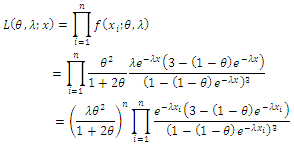 Then, the log likelihood function is given by
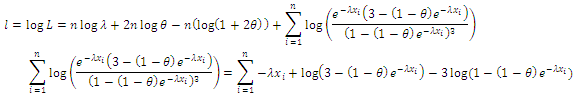 Thus
Thus To maximize
  taken first order partial derivatives of
  with respect to
  and equating the results equations to zeros and solve them.Taking derivatives to
  with respect to
  respectively, one get:
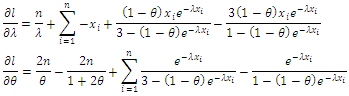 By equating
  and
and  to zero and solving for
  and
and  the MLE of theses parameters are numerically solutions of the following two equations:
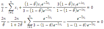
6.2. Maximum Likelihood Estimation for (CWTNDL) as Follows
The estimators of unknown parameters of the CWTNDL model are obtained based on maximum likelihood (ML) method. Let  be a random sample of size
  from CWTNDL, with set a parameters
  the likelihood function of the density is given by,
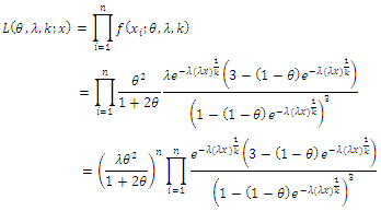 Then, the log likelihood function is given by
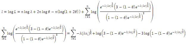 Thus
Thus To maximize
  taken first order partial derivatives of
  with respect to
  and equating the results equations to zeros and solve them.Taking derivatives to
  with respect to
  respectively, one get:
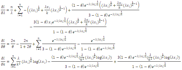 By equating
 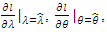 and
and  to zero and solving for
  the MLE of theses parameters are numerically solutions of the following three equations:
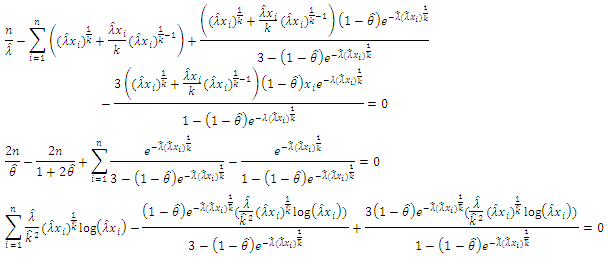
6.3. Maximum Likelihood Estimation for (CLTNDL) as Follows
The estimators of unknown parameters of the CLTNDL model are obtained based on maximum likelihood (ML) method. Let  be a random sample of size
  from CETNDL, with set a parameters
  the likelihood function of the density is given by,
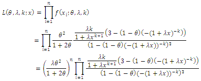 Then, the log likelihood function is given by
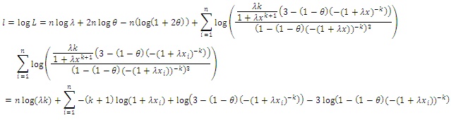 Thus
Thus To maximize
  taken first order partial derivatives of
  with respect to
  and equating the results equations to zeros and solve them.Taking derivatives to
  with respect to
  respectively, one get:
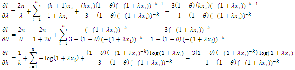 By equating
 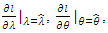 and
and  to zero and solving for
  the MLE of theses parameters are numerically solutions of the following three equations:
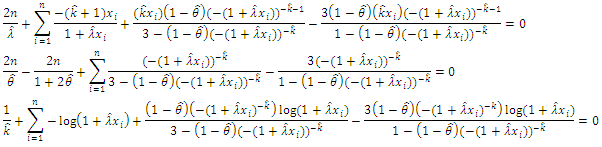
Table (1). Maximum likelihood, standard errors and associated asymptotic confidence interval estimates for CETNDL, CLTNDL and CWTNDL distributions based in series and systems given data set I
 |
| |
|
Table (2). Maximum likelihood, standard errors and associated asymptotic confidence interval estimates for CETNDL, CLTNDL and CWTNDL distributions based in series and systems given data set II
 |
| |
|
7. Application
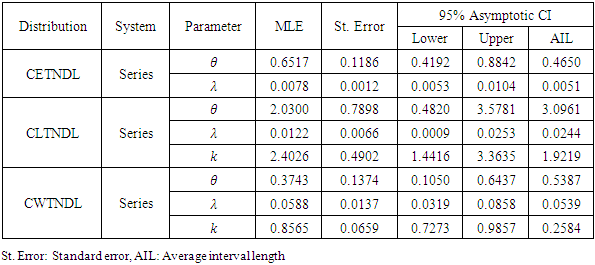
In this section we present an application of the Complementary Exponential Truncated Natural Discrete Lindley Distribution, Complementary Weibull Truncated Natural Discrete Lindley Distribution and Complementary Lomax Truncated Natural Discrete Lindley Distribution to two real data sets and fit the Exponential Distribution, Weibull Distribution and Lomax Distribution. The first data set corresponding to remission times (in months) of a random sample of 128 bladder cancer patients given in Lee and Wang (2003). The data are given as follows: 0.08, 2.09, 3.48, 4.87, 6.94, 8.66, 13.11, 23.63, 0.20, 2.23, 3.52, 4.98, 6.97, 9.02, 13.29, 0.40, 2.26, 3.57, 5.06, 7.09, 9.22, 13.80, 25.74, 0.50, 2.46, 3.64, 5.09, 7.26, 9.47, 14.24, 25.82, 0.51, 2.54, 3.70, 5.17, 7.28, 9.74, 14.76, 26.31, 0.81, 2.62, 3.82, 5.32, 7.32, 10.06, 14.77, 32.15, 2.64, 3.88, 5.32, 7.39, 10.34, 14.83, 34.26, 0.90, 2.69, 4.18, 5.34, 7.59, 10.66, 15.96, 36.66, 1.05, 2.69, 4.23, 5.41, 7.62, 10.75, 16.62, 43.01, 1.19, 2.75, 4.26, 5.41, 7.63, 17.12, 46.12, 1.26, 2.83, 4.33, 5.49, 7.66, 11.25, 17.14, 79.05, 1.35, 2.87, 5.62, 7.87, 11.64, 17.36, 1.40, 3.02, 4.34, 5.71, 7.93, 11.79, 18.10, 1.46, 4.40, 5.85, 8.26, 11.98, 19.13, 1.76, 3.25, 4.50, 6.25, 8.37, 12.02, 2.02, 3.31, 4.51, 6.54, 8.53, 12.03, 20.28, 2.02, 3.36, 6.76, 12.07, 21.73, 2.07, 3.36, 6.93, 8.65, 12.63, 22.69.Table 4.3 The MLEs of the parameters, the values of K-S statistic, BIC, AIC, HQIC, NLC and P-Value are summarized in Table (1, 2 and 3). From this tables, we note that the TNL-Exponential distribution is better than the Exponential distribution in terms of fitting to this data, that the TNL-Weibull distribution is better than the Weibull distribution in terms of fitting to this data and the TNL-Lomax distribution is better than the Lomax distribution in terms of fitting to this data.The AIC (Akaike Information Criterion) is given by where
where  is the number of estimated parameters.where is the number of the sample size in the model. The Bayesian information criterion (BIC) is given by
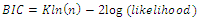 where
where  is the sample size of the training set. The lower BIC score signals a better mode.The second data set is obtained from: Leukemia 33, the data are:c(194, 413, 90, 74, 55, 23, 97, 50, 359, 50, 130, 487, 102,15, 14, 10, 57, 320, 261, 51, 44, 9, 254, 493, 18, 209, 41,58, 60, 48, 56, 87, 11, 102, 12, 5, 100, 14, 29, 37, 186,29, 104, 7, 4, 72, 270, 283, 7, 57, 33, 100, 61, 502, 220,120, 141, 22, 603, 35, 98, 54, 181, 65, 49, 12, 239, 14, 18,39, 3, 12, 5, 32, 9, 14, 70, 47, 62, 142, 3, 104, 85, 67,169, 24, 21, 246, 47, 68, 15, 2, 91, 59, 447, 56, 29, 176,225, 77, 197, 438, 43, 134, 184, 20, 386, 182, 71, 80, 188,230, 152, 36, 79, 59, 33, 246, 1, 79, 3, 27, 201, 84, 27,21, 16, 88, 130, 14, 118, 44, 15, 42, 106, 46, 230, 59, 153,104, 20, 206, 5, 66, 34, 29, 26, 35, 5, 82, 5, 61, 31, 118,326, 12, 54, 36, 34, 18, 25, 120, 31, 22, 18, 156, 11, 216,139, 67, 310, 3, 46, 210, 57, 76, 14, 111, 97, 62, 26, 71,39, 30, 7, 44, 11, 63, 23, 22, 23, 14, 18, 13, 34, 62, 11,191, 14, 16, 18, 130, 90, 163, 208, 1, 24, 70, 16, 101, 52,208, 95).The MLEs of the parameters the values of K-S statistic, BIC, AIC, HQIC, NLC and P-Value are summarized in Table (1, 2 and 3). From this tables, we note that the TNL-Exponential distribution is better than the Exponential distribution in terms of fitting to this data, that the TNL-Weibull distribution is better than the Weibull distribution in terms of fitting to this data and the TNL-Lomax distribution is better than the Lomax distribution in terms of fitting to this data.
Table (1). Comparison between the Exponential Distribution and Complementary Exponential Truncated Natural Discrete Lindley Distribution
 |
| |
|
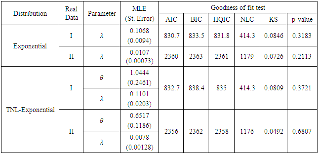
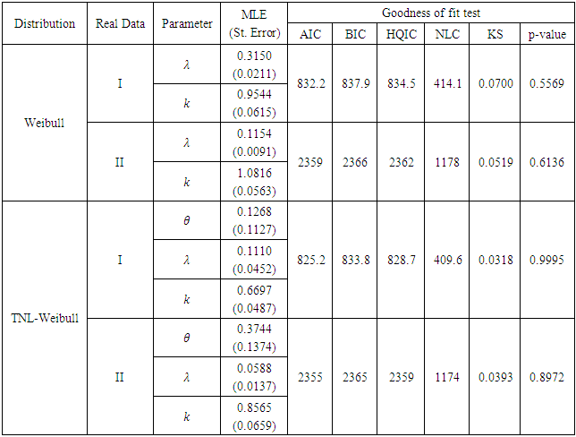
The MLEs of the parameters, the values of K-S statistic, BIC, AIC, HQIC, NLC and P-Value are summarized in Table (1). From this table, we note that the TNL-Exponential distribution is better than the Exponential distribution in terms of fitting to this data.Table (2). Comparison between the Weibull Distribution and Complementary Weibull Truncated Natural Discrete Lindley Distribution
 |
| |
|
The MLEs of the parameters, the values of K-S statistic, BIC, AIC, HQIC, NLC and P-Value are summarized in Table (2). From this table, we note that the TNL-Weibull distribution is better than the Weibull distribution in terms of fitting to this data.Table (3). Comparison between the Lomax Distribution and Complementary Lomax Truncated Natural Discrete Lindley Distribution
 |
| |
|
The MLEs of the parameters, the values of K-S statistic, BIC, AIC, HQIC, NLC and P-Value are summarized in Table (3). From this table, we note that the TNL-Lomax distribution is better than the Lomax distribution in terms of fitting to this data.
8. Conclusions
In this chapter a three new families of lifetime distributions called the complementary exponential truncated natural discrete Lindley distribution (CETNDL), the complementary Weibull truncated natural discrete Lindley distribution (CWTNDL) and the complementary Lomax truncated natural discrete Lindley distribution (CLTNDL) is introduced, this family is obtained by compounding the exponential distribution with truncated natural discrete Lindley distribution, compounding the Weibull distribution with truncated natural discrete Lindley distribution and compounding the Lomax distribution with truncated natural discrete Lindley distribution. It is observed the (CETNDL), (CWTNDL) and (CLTNDL) can have increasing, decreasing, constant, bathtub and upside-down hazard rate functions which are eligible for data analysis purposes. Several properties of the (CETNDL), (CWTNDL) and (CLTNDL) distributions such as quantiles, median, mean deviations, moments, Lorenz and Bonferroni curves,. This family contains several new distributions such as complementary exponentiated truncated natural discrete Lindley distribution, complementary Weibull logarithmic truncated natural discrete Lindley distribution, complementary weibull geometric truncated natural discrete Lindley distribution and, complementary Weibull Poisson truncated natural discrete Lindley distribution, cdf, pdf, hazard function of these special sub-models are presented. The method of maximum likelihood is used for estimating the model parameters. Finally the complementary exponential truncated natural discrete Lindley (CETNDL), the complementary Weibull truncated natural discrete Lindley (CWTNDL) and the complementary Lomax truncated natural discrete Lindley (CLTNDL) series models are fitted to real data sets to show the flexibility and potentiality of the proposed of distributions.
ACKNOWLEDGMENTS
The authorswould like to thank the Editor and the anonymous referees for very careful reading and valuable comments which greatly improved the paper.
Disclosure Statement
No potential conflict of interest was reported by the authors.
References
| [1] | Adamidis, K. and Loukas, S. (1998). A lifetime distribution with decreasing failure rate. Statistics and Probability Letters, 39, 35–42. |
| [2] | Dugas, M. R., & Samaniego, F. J. (2007). On optimal system designs in reliability-economics frameworks. Naval Research Logistics (NRL), 54(5), 568-582. |
| [3] | J.J. Barlow A.P. Mathias R. Williamson D.B. Gammack. (1963). A simple method for the quantitative isolation of undegraded high molecular weight ribonucleic acid. |
| [4] | LAGAKOS, S. W., BARRAJ, L. M., & Gruttola, V. D. (1988). Nonparametric analysis of truncated survival data, with application to AIDS. Biometrika, 75(3), 515-523. |
| [5] | Navarro, J., Samaniego, F. J., Balakrishnan, N., & Bhattacharya, D. (2008). On the application and extension of system signatures in engineering reliability. Naval Research Logistics (NRL), 55(4), 313-327. |
| [6] | Samaniego, F. J., Balakrishnan, N., & Navarro, J. (2009). Dynamic signatures and their use in comparing the reliability of new and used systems. Naval Research Logistics (NRL), 56(6), 577-591. |
| [7] | Nelson, W. (1982). Applied Life Data Analysis. New York: John Wiley & Sons, Inc. |

 Abstract
 Reference
 Full-Text PDF
 Full-text HTML