-
Paper Information
- Paper Submission
-
Journal Information
- About This Journal
- Editorial Board
- Current Issue
- Archive
- Author Guidelines
- Contact Us
International Journal of Probability and Statistics
p-ISSN: 2168-4871 e-ISSN: 2168-4863
2021; 10(2): 27-45
doi:10.5923/j.ijps.20211002.01
Received: May 8, 2021; Accepted: Jun. 2, 2021; Published: Jun. 15, 2021

Berry-Esseen Type Bound in Partially Linear Regression Model under Mixing Sequences
 Abstract
 Reference
 Full-Text PDF
 Full-text HTML
Sallieu Kabay Samura
Department of Mathematics and Statistics, Fourah Bay College, University of Sierra Leone, Sierra Leone
Correspondence to: Sallieu Kabay Samura , Department of Mathematics and Statistics, Fourah Bay College, University of Sierra Leone, Sierra Leone.
| Email: |  |
Copyright © 2021 The Author(s). Published by Scientific & Academic Publishing.
This work is licensed under the Creative Commons Attribution International License (CC BY).
http://creativecommons.org/licenses/by/4.0/

It is well-known that the confidence intervals of  and
and  in partially linear regression model lie in the limit distributions of their estimators. However the accuracy of the confidence intervals depends on how fast the theoretical distributions of the estimators converge to their limits. As a results, Berry-Esseen type bounds can be used to assess the accuracy. The aim of this paper is to study the Barry-Esseen type bounds for the estimators of
  and
and  in the partially linear regression model with
  satisfying
  with
with  and
and  being stationary
  -mixing random variables. By choosing suitable weighted functions, the Berry-Esseen type bounds for the estimators
  and
and  can achieve
  and
and  respectively. Simulation studies are conducted to demonstrate the performance of the proposed procedure.
Keywords:
Partially linear model, Berry-esseen bound,  -mixing sequence
Cite this paper: Sallieu Kabay Samura , Berry-Esseen Type Bound in Partially Linear Regression Model under Mixing Sequences, International Journal of Probability and Statistics , Vol. 10 No. 2, 2021, pp. 27-45. doi: 10.5923/j.ijps.20211002.01.
Article Outline
1. Introduction
- Partially linear regression model is a combination of linear and nonparametric parts in which the relationship between the response and some explanatory variables are linear whereas the other predictors are emerged in the model in unspecified association form. Opsomer and Ruppert (1999) argued for the advantage of partially linear regression model, including that there is less worry of overfitting, that they are more easily interpretable, and that the estimator is more efficient for the parametric components. Also, various estimation and variable selection methods for the partially linear regression model have been developed which we refer to, Horowitz (2009), Liu et al. (2011), Roozbeh et al. (2012), Amini and Roozbeh (2016), Roozbeh and Arashi (2016), Roozbeh (2018) and Amini and Roozbeh (2019) to mention a few.Since its introduction by Engle et al. (1986), partially linear regression models have been studied by many authors. For example, Heckman (1986), Rice (1986), Chen (1988) and Speckman (1988) studied the consistency properties of the estimator of
 under different assumptions. Schick (1996) and Liang and Härdle (1997) extended the root n consistency and asymptotic results for the case of heteroscedasticity. Härdle et al. (2000) provided a good comprehensive reference of the partially linear model. Chen et al. (1998) and Gao et al. (1994) established the strong consistency and asymptotic normality, respectively, for the least squares estimators and weighted least-squares estimator (WLSE, for short) of
  based on nonparametric estimates
  and
and  You et al. (2007) further studied the model and developed an inferential procedure which includes a test of heteroscedasticity, a two-step estimator of
  , mean square errors of
  and
and  and a bootstrap goodness of fit test. If
  then the model boils down to the heteroscedastic linear model, whose asymptotic properties of the WLSE of
  were studied by Carroll (1982), Robinson (1987) and Carroll and Härdle (1989), respectively.In this paper, we will further study the limit behaviors of the estimators in the partially linear regression model under
  -mixing random variables, the concept of which was first introduced by Bradley (1985) as follows.Let
  be a sequence of random variables defined on a fixed probability space
  . Denote
  and
and  . Let
. Let  and
and  be positive integers. Write
  . Given
  -algebras
  and
and  in
in  , let
, let where
where  and
and  . Define the
  -mixing coefficients by
 Definition 1.1. A sequence
  of random variable is said to be
  -mixing if
  as
as  Since the concept of
  -mixing was introduced by Bradley (1985), many limit theorems were established. Bradley (1985) discussed central limit theorems under absolute regularity for
  -mixing sequences. Shao (1993) established limit theorems of
  -mixing sequences; Cai (1991) obtained strong consistency and rates for recursive nonparametric conditional probability density estimators under
  -mixing conditions; Lu and Lin (1997) gave the bounds of covariance of
  -mixing sequences; Shen and Zhang (2011) studied some convergence theorems for
  -mixing random variables, and obtained some new strong laws of large numbers for weighted sums of
  -mixing random variables; Gao (2016) investigated the
  -mixing sequences which are stochastically dominated, and presented some strong stability; Yu (2016) showed the Resenthal-type inequality of the
  -mixing sequences, and investigated the strong convergence theorems.The aim of this paper is to further study the Barry-Esseen type bounds for the estimators of
  and
and  in the partially linear regression model (2.1) with
  satisfying
  with
with  and
and  being stationary
  -mixing random variables. By choosing suitable weighted functions, the Berry-Esseen type bounds for the estimators
  and
and  can achieve
  and
and  respectively.This work is organised as follows: In Section 2, we recall the partially linear regression model and construct the partial least squares estimator for both the parametric and non-parametric components. The main results and numerical analysis (simulations and real data) are presented in Section 3. The proofs of the main results are provided in Section 4.Throughout this paper, the symbols
  denote positive constants whose values may be different in different places. Let
  and
and  be the indicator function of the set
  . Let
. Let 
2. Model and Estimation
- Consider the following partially linear regression model:
 | (2.1) |
 is an unknown parameter of interest,
  are nonrandom design points,
  are the response variables,
  are random errors,
  is an unknown functions defined on closed interval [0,1].If
  is the true parameter, then model (2.1) is reduced to a nonparametric regression model
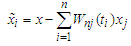
  Since
Since  we have
 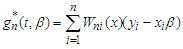 . Using the least squares method, we obtain
  of
of  by minimizing
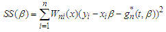 The minimizer is found to be
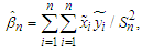 | (2.2) |
 ,
, and
and 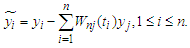 Then based on
  we defined the nonparametric function
  by
by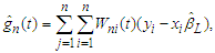 | (2.3) |
 on [0,1] such that
  and(i)
 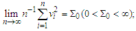 (ii)
(ii)  A2.
A2.  and
and  are defined on [0,1] and satisfy Lipschitz condition of order 1.A3. The probability weight function
  are defined on [0,1] and satisfy
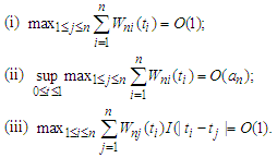 A4.
A4.  for some
  A5. There exist positive integers
  and
and  such that


 A6. The spectral density
  of
of  satisfies that
  Remark 2.1 Conditions (A1)-(A3) have been used frequently by many authors. For example, Gao et al. [1996], Sun et al. [2002], You et al. [2005], Liang et al. [2006], You and Chen [2007] and so on. (A4) is adopted in Sun et al. [2002], You et al. [2005], Liang et al. [2006], Liang and Fan [2009] and so forth. Moreover, if functions
  and
and  satisfy a Lipschitz condition of order 1 on [0,1], then (A3) (iii) implies that
  and
and 
3. Main Results and Numerical Analysis
3.1. Main Results
- In this subsection, we present the Berry-Esseen type bounds for the estimators
 ,
,  . We first introduce some notations which will be used in the theorem below.
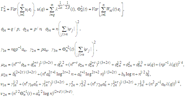 Theorem 3.1. Let
  be a mean zero
  -mixing sequence, with
  , where
  and
and  Suppose that conditions
  are satisfied,
  and
and  for some
  . Let
. Let  for some
  Assume that
 . Then, for
  and any
  we have
 | (3.1) |
 and
and  where
where  and
and  for some
  . Let
. Let  ,
,  for some
  and
and  for some
  ,
,  Then
Then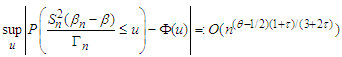 Theorem 3.2. Suppose that the conditions in theorem 3.1 hold. Let
 and
and  If
If  and
and  converge to zero, then
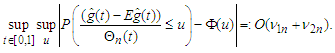 | (3.2) |
 for some
  and
and  Suppose that
  hold with
  for each
  and
and  for some
  Let
Let 
 for some
  and
and  for some
  , then
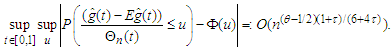
3.2. Numerical Simulation
- In this subsection, We carry out a simulation to study the asymptotic normality of the estimators
 and
and  , respectively. The observations are generated for the following model:
 where
where  is an AR(1) type process
  with
with  be an MA(1) process specified by
  and
and  , for
, for 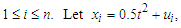 where
where  and
and  for
for  Here, we choose the nearest neighbor weights to be the weight functions
  For any
  we rewrite
 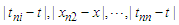 as follows
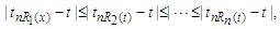 if
if  , then
  is permutated before
  when
when  . Take
  and defined the nearest neighbor weight function as follows:
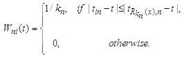 We generate the observed data with sample size
  as
as  and
and  respectively. We used R software to compute
  and
and 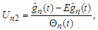 and obtained the Q-Q plots of
  and
and  respectively, based on 500 replications.
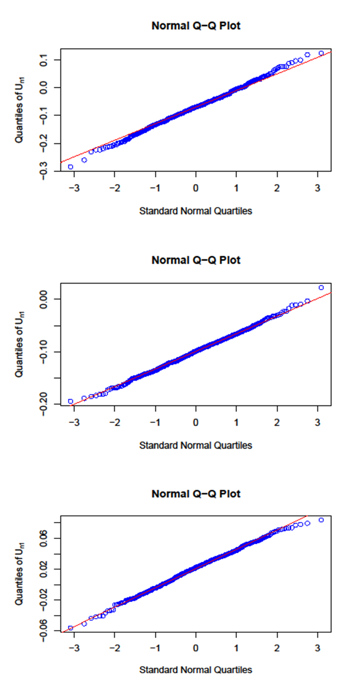 | Figure 1. Q-Q plot of  with with  =50, 100 and 150, respectively =50, 100 and 150, respectively |
 | Figure 2. Q-Q plot of  with with  =50, 100 and 150, respectively =50, 100 and 150, respectively |
4. Proofs of the Main Results
- We first introduce several lemmas which will be used to prove the main results of the paper.Lemma 3.1. (cf. Yu, 2016) Let
 be a sequence of
  -mixing random variables with
  ,
,  for some
  and
and  , where
  and
and  Assume that
 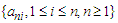 is an array of real numbers. Then there exists a positive constant
  depending only on
  and
and  such that
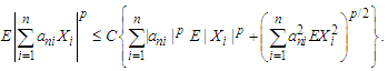 Lemma 3.2. (Liang and Fan, 2009) Let
  be random variables. For positive numbers
  we have that
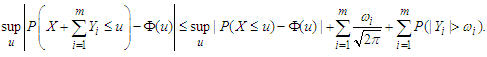 Lemma 3.3. (Lu and Lin (1997)) Let
  be a sequence of
  -mixing random variables. Suppose that
  and
and  where
where  and
and  Then
Then Lemma 3.4. Let
  be a sequence of
  -mixing random variables. Suppose that p and q are two positive integers. Let
 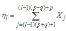 for
for  Then for any
 Proof. It is easily checked that
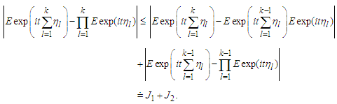 | (4.1) |
 we have
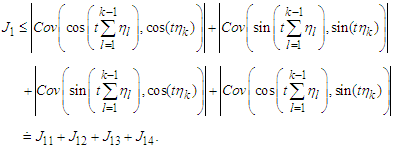 | (4.2) |
 that
that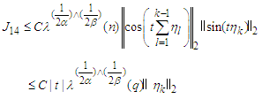 | (4.3) |
 | (4.4) |
 and hence applying Lemma 3.3 and invoking again the inequality
  we find that
 | (4.5) |
 | (4.6) |
 Proceeding in this manner, we obtain
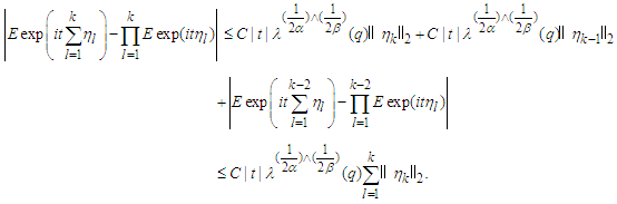 This completes the proof of the lemma.Lemma 3.5. Let
  be an array of real numbers such that
  and
and  where
where  are some positive numbers. Suppose that
  for some
  and
and  for some
  Then for any
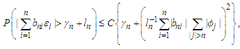 and
and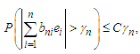 where
where  are positive numbers and
  for some
  and any
  Proof. We only prove the first inequality, and the second one is completely analogous. According to the definition of
  we have that
 By
By  and Markov's inequality, we have
 Note that
 Applying Lemma 3.1 with
 Noting that
  and
and  implies
  we have
 Where the inequality in the last line above follows from
 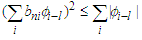 and changing the order of simulation. The proof is completed.Lemma 3.6. Under the assumptions of Theorem 2.1, the following statements hold.
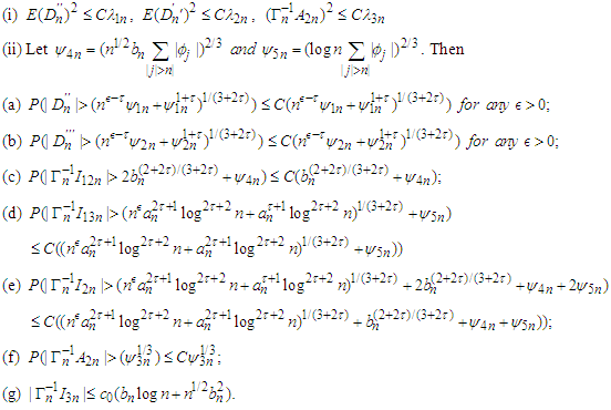 Proof. (i) Applying Lemma 3.2 with
  and
and  inequality, we have by
 for
for  (A1) (iii) and (1.2) that
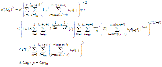 | (4.7) |
 inequality again that
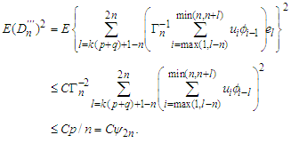 Moreover, we have by
  and (A1) (iii) again and
  that
that Hence (i) has been proved.(ii) The inequalities (a)-(e) can be proved by applying Lemma 3.5. Now we will verify them one by one.(a) Noting by (A1) (iii) that
  and
and  the result follows immediately form Lemma 3.5.(b) Similarly, noting additionally that
  we have by Lemma 3.5 again that the result follows.(c) Note that
  Therefore, we have
  Let
Let  we have Lemma 3.5 again that
 (d) Observe that
  Utilizing the Abel Inequality (see Mitrinovic, 1970, Theorem 1, p.32), we have by (A1) and (A3) that
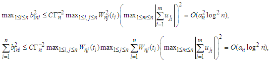 and
and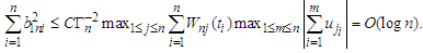 Thus the result follow from Lemma 3.5 immediately.(e) It follows
 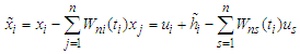 that
that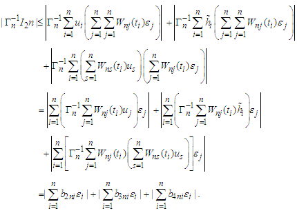 Similar to the proofs of (c) and (d), we have
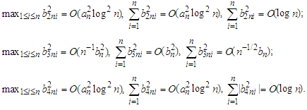 Choosing
  we have by Lemma 3.5 again that
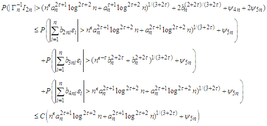 (f) The inequality (f) can be derived immediately by (i) and Markov's inequality.(g) It follows from the Abel Inequality and Remark 2.1 again that
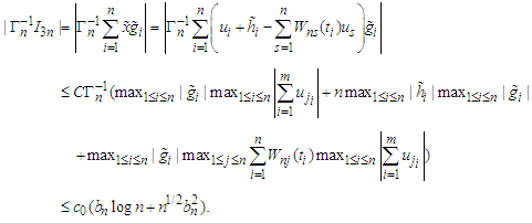 The prove is completed.Lemma 3.7 Let
  Then under the assumption of Theorem 3.1, we have
 Proof. Similar to Lemma 3.6 in Liang and Fan (2009), we can complete the proof of the lemma. The details are omitted.Assume that
  are independent random variables and
  has the same distribution as that of
  for each
  Let
Let  then
then  Lemma 3.7 Under the assumptions of Theorem 3.1, we have
 Proof. We have by Berry-Esseen inequality (Petrov, 1995, p.154, Theorem 5.7) that
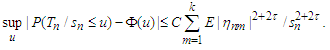 Applying Lemma 3.3 with
  and noting that
  we have by choosing
  that
that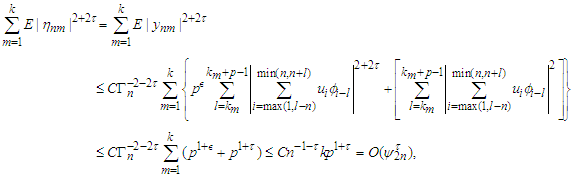 which together with
  from Lemma 3.7 yields that
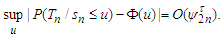 The prove is completed.Lemma 3.8 Under the assumptions of Theorem 3.1, we have
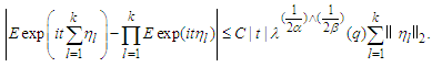
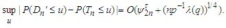 Proof. Suppose that
  are characteristic functions of
  respectively.We have by Esseen inequality (Petrov, 1995, p.146, Theorem 5.3) that for any
 Applying Lemma 3.4 with
  and Lemma 3.2 with
  and similar to the proof of (3.2), we have by
  that
that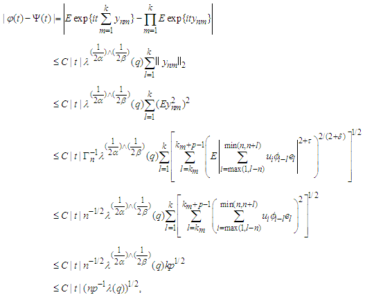 which implies that
 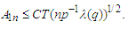 On the other hand, from Lemma 3.7 and we have
 which derives that
  By choosing
  we can obtain that
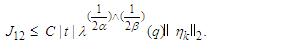
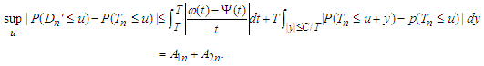
 This completes the proof of the lemma.Proof of Theorem 3.1 We can observe that
 It is easy to show that
 and
and By changing the order of summation, we obtain that
 Let
Let  Denote
 The we have that
 It follows from Lemma 3.7-3.9 that
 Consequently, from (3.1), Lemma 3.1 and Lemma 3.6, we have
 The proof of the theorem is completed.To prove Theorem 2.2, we need the following lemmas.Lemma 3.8 Under the assumption of Theorem 2.2, the following statements hold.
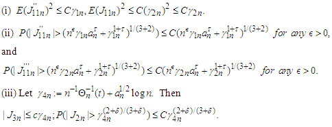 Furthermore, if
  for some positive numbers
  then
then Proof. (i) Similar to the proof of (3.2), we have by
  that
that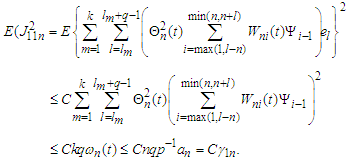 Similarly,
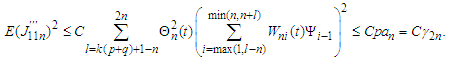 Noting that
  analogous to the proof of (3.3) we have
  (ii) Noting that
 and
and the first inequality follows immediately form Lemma 3.5.Similarly, noting that
 we can also get the second one from Lemma 3.5.(iii) Observe that
  in Theorem 2.1, the proof of (iii) can be easily obtained by following the proof of Lemma 3.9 in Liang and Fan (2009). The details are omitted here.Lemma 3.11. Let
  Then under the assumptions of Theorem 2.2, we have
 Proof. Similar to the proof of Lemma 3.10 in Liang and Fan (2009), we can prove the lemma.The details are omitted.Assume that
  are independent random variables and
  has the same distribution as that of
  for each
  Let
Let 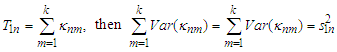 .Lemma 3.12 Under the assumptions of Theorem 2.2, we have
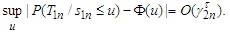 Proof. Note that
 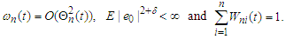 Similar to the proof of Lemma 3.8, we have by Lemma 3.3,
 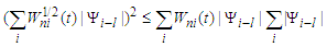 and changing the order of summation that
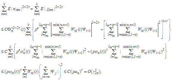 which together with
  from Lemma 3.11 yields that
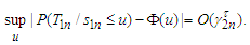 The proof is completed.Lemma 3.13 Under the assumptions of Theorem 2.2, we have
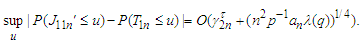 Proof. Suppose that
  are the characteristic functions of
  respectively. Similar to the proof of Lemma 3.9, we have
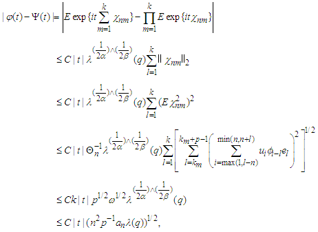 together with Lemma 3.11 and 3.12 yield that
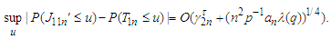 This completes the proof of the lemma.Proof of Theorem 3.1 We have that
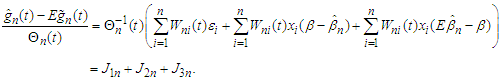 Note that
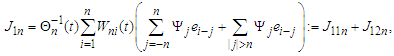 and
and Similar to the decomposition for
  we denote
 Then we have that
 we have by Lemma 3.11-3.13 that
 which together with (3.4), Lemma 3.1 and Lemma 3.10 yields that
 The proof is completed.