Kelechukwu C. N. Dozie , Hope I. Mbachu, Mirian C. Raymond
Department of Statistics Imo State University Owerri, Imo State, Nigeria
Correspondence to: Kelechukwu C. N. Dozie , Department of Statistics Imo State University Owerri, Imo State, Nigeria.
| Email: |  |
Copyright © 2020 The Author(s). Published by Scientific & Academic Publishing.
This work is licensed under the Creative Commons Attribution International License (CC BY).
http://creativecommons.org/licenses/by/4.0/

Abstract
This paper examines the condition(s) under which the mixed model is the most appropriate model in descriptive time series analysis when trend-cycle component is linear. Since some existing studies have adequately characterized the additive model, the analyst is still exposed to the risk of wrongly using multiplicative model when mixed model should be used. Therefore, the aim of this study is to identify the series that admits mixed model. The method employed in this paper is the Buys-Ballot procedure developed for choice of model and choice of appropriate transformations, among other uses, based on row, column and over totals, means and variances of the Buys-Ballot table. Results show that, 1) the seasonal variance of the Buys-Ballot table, for the mixed model, a function of the slope and seasonal effect only. 2) the calculated values of the test statistic identified the mixed model correctly in 99 out the 100 stimulations.
Keywords:
Keywords Choice of Model, Time Series Decomposition, Mixed Model, Buys-Ballot Table
Cite this paper: Kelechukwu C. N. Dozie , Hope I. Mbachu, Mirian C. Raymond , The Analysis of Mixed Model in Time Series Decomposition, International Journal of Probability and Statistics , Vol. 9 No. 1, 2020, pp. 1-6. doi: 10.5923/j.ijps.20200901.01.
1. Introduction
The objective of time series decomposition is to separate the four time series components available in the series. That is, to de-compose an observed time series  into components, representing the trend
  , the seasonal
  , cyclical
  and irregular
  Kendal and Ord [9], Chatfield [2]. The models most commonly used to describe time series decomposition are theAdditive Model:
 | (1) |
Multiplicative Model:  | (2) |
and Mixed Model | (3) |
for short series, the trend component is jointly estimated into the cyclical Chatfield [2] and the observed time series  can be decomposed into the trend-cycle component
  , seasonal component
  and the irregular/residual component
  . Therefore, the decomposition models areAdditive Model:
  | (4) |
Multiplicative Model:  | (5) |
and Mixed Model  | (6) |
It is always assumed that the seasonal effect, when it exists, has period s, that is, it repeats after s time periods. | (7) |
For additive model, it is convenient to make assumption that the sum of the seasonal components over a complete period is zero, ie, | (8) |
Similarly, for multiplicative and mixed models, it equally convenient to make assumption that the sum of the seasonal components over a complete period is s. | (9) |
It is also assumed that the error term  is the Gaussian
  white noise for additive and mixed models, while for multiplicative model,
  is the Gaussian
  white noise and that
 It is assumed that (i) the appropriate model for decomposition is known; (ii) the study series satisfied the assumptions of the models. However, one of the greatest problems identified in the use of descriptive method of time series analysis is choice of appropriate model for decomposition of any study data. That is when to use any of the additive, multiplicative and mixed models for analysis is uncertain. And it is clear that; use of wrong model will definitely lead to erroneous estimates of the components. The emphasis of this paper is to identify the series that admits mixed model. This work is restricted to time series with linear using stimulated series of 100 data sets of 120 observations each stimulated from the mixed model and real life data on number of Hennessey drinks sold at Vandoz Enterprise, Owerri, Imo Stata, Nigeria for the period 2008 to 2017. Iwueze and Nwogu [7] provided a framework for choice of model and detection of seasonal effect in time series. The framework shows that the column (seasonal) variances of the Buys-Ballot table are, for the additive model, functions of only trend parameters and for multiplicative model, functions of the trend parameters and seasonal indices. In particular, when the trend-cycle component is linear, the column variances are constant for additive model, but contain the seasonal component for the multiplicative model. Therefore, choice between additive and multiplicative models reduces to test for constant variance to identify the additive model. Thus, they suggested that any of the test for constant variance can be used to identify a series that admits the additive model. This is an improvement of what is available in the literature. However, this approach can only identify the additive model, when the column variance is constant, but does not suggest to the analyst the alternative model when the variance is not constant. The implication of this is that when the test for constant variance says the appropriate model is not the additive model; an analyst still faces the challenge of choosing between mixed model and the multiplicative model.
1.1. Buys-Ballot Procedure for Time Series Decomposition
Iwueze, et al, [8] observed that, for time series which contain a seasonal effect, the overall mean  and seasonal means
  of the Buys – Ballot table are used to assess the effects either as a difference
  or the ratio
  That is, the deviation of the differences seasonal averages and the overall averages (additive model) from zero or the overall average from unity (multiplicative model) is used to assess the presence of seasonal effects. The Buys - Ballot table helps in the assessment of the trend – cycle and seasonal effect of time series data. The row means
  estimate trend, and the differences
  or the ratio
  between the column means
  and the overall mean
  estimate the seasonal effects. Chartfield [2] stated the use of the Buys - Ballot table for inspecting time series data for the presence of trend and seasonal effects. Iwueze and Nwogu [4] developed a new estimation procedure based on row, column and overall averages of the Buys - Ballot table. This method called Buys – Ballot estimation procedure uses the periodic mean
  and the overall mean
  to estimate the trend component. Seasonal means
 and the overall mean
  are used to estimate the seasonal indices. Fomby [3] presented various graphs suggested by the Buys – Ballot table for inspecting time series data for the presence of seasonal effects.
2. Methodology
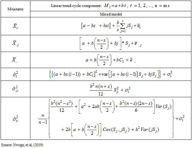
This section presents methodology adopted in this paper. The method adopted is the Buys-Ballot procedure for time series decomposition. This procedure has been developed for choice of transformation and choice of model, among other uses, based on the row, column and overall means and variances of the Buys-Ballot table. For detailed discussion of Buys-Ballot procedure, see Wei [11], Iwueze and Nwogu [4] and [5] Iwueze and Ohakwe [7]. The row, column and overall means and variance obtained by Nwogu, et al, [10] are given in Table 1. From Table 1, it is clear that the column variances of the Buys-Ballot table, a constant multiple of square of the seasonal effect only for the mixed model. Nwogu, et al, [10] proposed chi-square test for choice between the mixed and the multiplicative models is based on the column variances. The proposed test is able to distinguish a series that admits mixed model from a series that admit multiplicative model. According to them, the null hypothesis to be tested is and the appropriate model is mixed, against the alternative
 and the appropriate model is not mixed, where
 is the actual variance of the jth column.
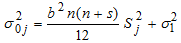 | (10) |
and  is the error variance, assumed equal to 1.They stated the statistic
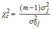 | (11) |
follows the chi-square distribution with  degrees of freedom, m is the number of observations in each column and
  is the seasonal lag (number of columns). They also showed that under the null hypothesis, the interval
 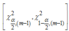 contains the statistic (11) with 100
  degree of confidence.
Table 1. Summary of Row, Column and Overall Means and Variances of Buys-Ballot for Mixed Model
 |
| |
|
2.1. Test for Constant Variance
Although there are many tests for constant variance, Bartlett’s test has been adopted in this work. Bartlett’s test is more robust. Bartlett’s test allows the comparison of variance of two or more samples to determine whether they are drawn from populations with equal variance. It is suitable for normally distributed data. To test the null hypothesis that the variances are equal, that is against the alternative
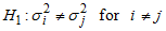 and at least one variance is different from othersBartlett [1] has shown that the statistic
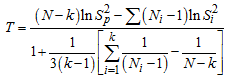 | (12) |
follows Chi-square distribution with  degrees of freedom. Using the parameters of the Buys-Ballot table,
 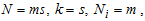 the statistic in (12) is then given as
 Where
Where  is the total number of observations,
  is the number of observations in each column and
  is length of the periodic interval.
3. Empirical Examples
The purpose of this section is to present empirical examples to illustrate the application of the proposed test by Nwogu, et al, [10]. The empirical example consists of both stimulated series from the mixed model and real life data.
3.1. Simulations Results from Mixed Model
The stimulated series used consist of 100 data sets of 120 observations each stimulated from mixed model 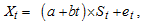 with
with 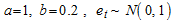 and
and  given in Table 2.
Table 2. Seasonal
 indices used in the simulation of series indices used in the simulation of series
 |
| |
|
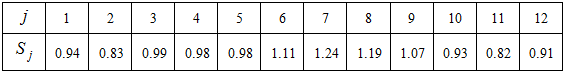
Each series of 120 observations has been arranged in a Buys-Ballot table as monthly data (s = 12) for 10 years (m = 10). The critical values, are for  degrees of freedom, equal to 2.7 and 19.0 and at 5% level of significance. The decision rule is to reject null hypothesis, if the calculated value of the statistic lie outside the interval otherwise do not reject it. When compared with the interval 2.7 and 19.0, the calculated values of the statistic in Table 3 lie within the interval in 99 out of the 100 simulations. The test identified the mixed model correctly in 99 out of the 100 stimulations.
 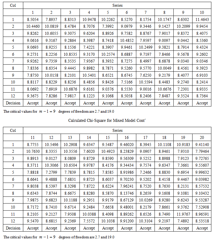 | Table 3. Calculated Chi-Square for Mixed Model |
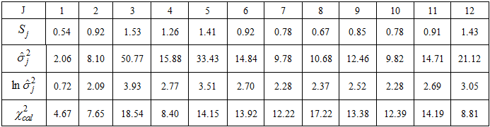
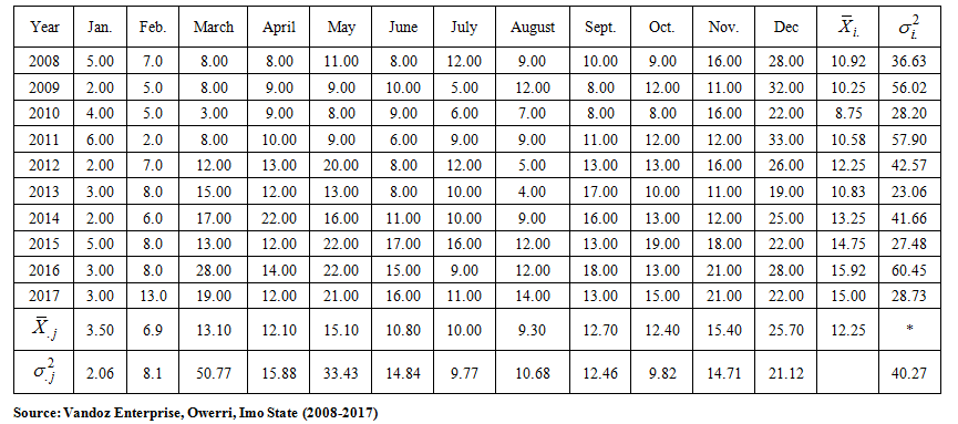
3.2. Real Life Data
The second empirical example is based on monthly data on number of Hennessey drinks sold at Vandoz Enterprise, in Owerri Municipal of Imo State for the period 2008 to 2017. The data is given in Appendix A while the time plot is in Figure 3.1. The column variances are shown in Table 4. The first step is to check whether the data admits additive model. To test the null hypothesis that the data admits additive model, the Bartlett’s test is used. The null hypothesis is rejected, if Tc is greater than the tabulated value, which for  level of significance and
  degrees of freedom equal to 19.7 or do not reject
  otherwise.
 | Figure 3.1. Time plot of the actual series on number of Hennessey drinks between (2008-2017) |
Table 4. Seasonal effects
 estimate of the column variance estimate of the column variance
 and Calculated Chi-square and Calculated Chi-square

 |
| |
|
From Appendix and Table 4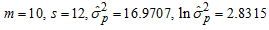 and
and 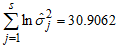 Hence,
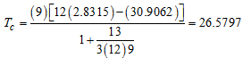 When compared with the critical value (19.7), Tc is greater, indicating that the data does not admit the additive model. Having confirmed that the data does not admit additive model, the choice now lies between mixed and multiplicative models. In other to choose between mixed and multiplicative models, the proposed test by Nwogu, et al, [10] is used. The null hypothesis that the data admits mixed model is rejected, if the statistic defined in (11) lies outside the interval
  which for m-1 = 9, equals (2.7 and 19.0) or do not reject
  otherwise.From Table 4,
 Hence, from (10)
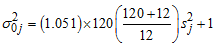 and the calculated values,
  given in Table 4 were obtained. When compared with the critical values (2.7 and 19.0), the calculated values of the statistic lie within the interval, indicating that the data admits mixed model.
4. Concluding Remarks
This paper has discussed the analysis of mixed model when trend-cycle component of time series is Linear. The emphasis is to identify the series that admit mixed model. The method adopted is Buys-Ballot procedure developed for choice model and choice of appropriate transformation, among others uses, based on row, column and overall totals, means and variances of Buys-Ballot table. Result from calculated value of the proposed test statistic shows that, the test identified mixed model correctly in 99 out of the 100 simulation In considering the mixed model, the residuals are assumed to be (i) uncorrelated; and (ii) normally distributed with mean equal to zero and constant variance. Cases, in which these assumptions are not met, are recommended for further investigation.
Appendix
 | Buys-Ballot table on number of Hennessey drink at Vandoz Enterprise (2008-2017) |
References
| [1] | Bartlett, M. S. (1937). Properties of Sufficiency and Statistical Tests. Proceedings of the Royal Statistical Society, Series A 160, 268-282 JSTOR 96803. |
| [2] | Chatfield, C. (2004). The analysis of time Series: An introduction. Chapman and Hall, /CRC Press, Boca Raton. |
| [3] | Fomby, T.B (2008). Buys–Ballot plots: graphical methods for detecting seasonality in time series. faculty.smu.edu/tfomby/eco5375/data/…/Buys%20Ballot%plotpdf. |
| [4] | Iwueze, I. S. & Nwogu E.C. (2004). Buys-Ballot estimates for time series decomposition, Global Journal of Mathematics, 3(2), 83-98. |
| [5] | Iwueze, I. S. & Nwogu, E.C. (2005). Buys-Ballot estimates for exponential and s-shaped curves, for time series, Journal of the Nigerian Association of Mathematical Physics, 9, 357-366. |
| [6] | Iwueze, I. S. & Nwogu, E.C. (2014). Framework for choice of models and detection of seasonal effect in time series. Far East Journal of Theoretical Statistics 48(1), 45– 66. |
| [7] | Iwueze, I. S. & Ohakwe, J. (2004). Buys-Ballot estimates when stochastic trend is quadratic. Journal of the Nigerian Association of Mathematical Physics, 8, 311-318. |
| [8] | Iwueze, I.S., Nwogu, E.C., Ohakwe, J. & Ajaraogu. J.C (2011). Uses of the Buys – Ballot table in time series analysis. Applied Mathematics Journal 2, 633 –645. |
| [9] | Kendal, M. G. & Ord, J. K. (1990). Time Series (3rded.). Charles Griffin, London. |
| [10] | Nwogu, E.C, Iwueze, I.S. Dozie, K.C.N. & Mbachu, H.I (2019). Choice between mixed and multiplicative models in time series decomposition. International. |
| [11] | Wei, W. W. S (1989). Time series analysis: Univariate and multivariate methods, Addison-Wesley publishing Company Inc, Redwood City. |

 Abstract
 Reference
 Full-Text PDF
 Full-text HTML