Akintunde Mutairu Oyewale 1, Chigozie Kelechi Acha 2, Agunloye Oluokun Kasali 3, Eriobu Nkiru Obioma 4, Oyekunle Janet Olufunmike 1, Abdulazeez Ismail Adeyinka 1
1Department of Statistics, School of Applied Sciences the Federal Polytechnic, Ede, Osun State, Nigeria
2Michael Okpara University of Agriculture, Umudike, Abia State, Nigeria
3Department of Mathematics, Faculty of Science Obafemi Awolowo University, Ile-Ife, Osun State, Nigeria
4Department of Statistics, Faculty of Physical Science, Nnamdi Azikiwe University, Awka, Anambra State
Correspondence to: Akintunde Mutairu Oyewale , Department of Statistics, School of Applied Sciences the Federal Polytechnic, Ede, Osun State, Nigeria.
| Email: |  |
Copyright © 2019 The Author(s). Published by Scientific & Academic Publishing.
This work is licensed under the Creative Commons Attribution International License (CC BY).
http://creativecommons.org/licenses/by/4.0/

Abstract
Foreign exchange is one of the most important financial instruments very volatile and chaotic in nature. Nowadays, the role of the foreign exchange market is becoming more and more important in the financial markets around the world; it remains the only instruments worldwide to measure the standard of living, Economic performance and country standing among the committee of nations. The foreign exchange market which is an over-the-counter market is used for the trading of currencies. It makes the foreign exchange market the largest and most liquid market among the financial markets. Necessary mathematical frame work was put in place, this was illustrated with data from record of Central Bank of Nigeria through their official website. Through this the performance of nonlinear threshold models in forecasting the exchange rate of Nigeria in relation to United States of American dollar as bench mark. The software used for the analysis was Econometrics View (E-view). Stationarity tests were carried out before the analysis, (the original data was not stationary, but at first difference it was stationary, thereafter comprehensive data analysis was performed). The forecasting results indicate that SETAR models did not outperform Random Walk in any period. TAR models offered promising results in the period. This study supports the general belief that the exchange rates are chaotic, volatile and very difficult to forecast and this applies to Exchange rate system of Nigeria as it is the case in the developed world.
Keywords:
Forecasting, Stationarity test, Exchange rate, Nonlinearity, SETAR, TAR
Cite this paper: Akintunde Mutairu Oyewale , Chigozie Kelechi Acha , Agunloye Oluokun Kasali , Eriobu Nkiru Obioma , Oyekunle Janet Olufunmike , Abdulazeez Ismail Adeyinka , Exchange Rate Forecasting Using Non-linear Threshold Models, International Journal of Probability and Statistics , Vol. 8 No. 2, 2019, pp. 30-36. doi: 10.5923/j.ijps.20190802.02.
1. Introduction
Foreign exchange is one of the most important financial instruments. Nowadays, the role of the foreign exchange market is becoming more and more important in the financial markets around the world. The foreign exchange market which is an over-the-counter market is used for the trading of currencies. The trading is happening 24 hours a day around the world and a great number of currencies is being transacted every hour. It makes the foreign exchange market the largest and most liquid market among the financial markets.There are so many studies on exchange rate forecasting carried out worldwide. Until now, there are a lot of forecasting models, each having its point of strengths and weaknesses used in exchange rate forecasting, such study include ARIMA model (Tseng, 2001), [19], Least Squared model [10] or Purchasing Power Parity model and [3]. [13] used ARIMA model for forecasting inflation in Irish, [14] used Arima model for forecasting stock price. ARIMA is also used for predicting stock price in the research of [12], [11]. It is also used for forecasting the price of gold [8].According to [1] Triennial Survey, turnover in global foreign exchange markets averaged $5.1 trillion per day. This is down from $5.4 trillion in April 2013, a month which had seen heightened activity in Japanese yen against the background of monetary policy developments at that time. In addition, exchange rate movements are used to compare influence of the previous surveys on the current year. In particular, the appreciation of the US dollar between 2013 compared with 2016. When valued at constant (April 2016) exchange rates, turnover increased slightly, by about 4% between April 2016 and April 2013. Nevertheless, the latest developments contrast with the strong growth in turnover observed between Triennial Surveys since 2001.The foreign exchange rate has two main uses. Firstly, it allows the businesses to exchange its currency to a target currency in the determined foreign exchange rate. Thus, it benefits the global trade and investment. Secondly, it also provides the speculation and expedites the carry trade, in which there are substantial profits available. However, there also exists high risk in the speculation.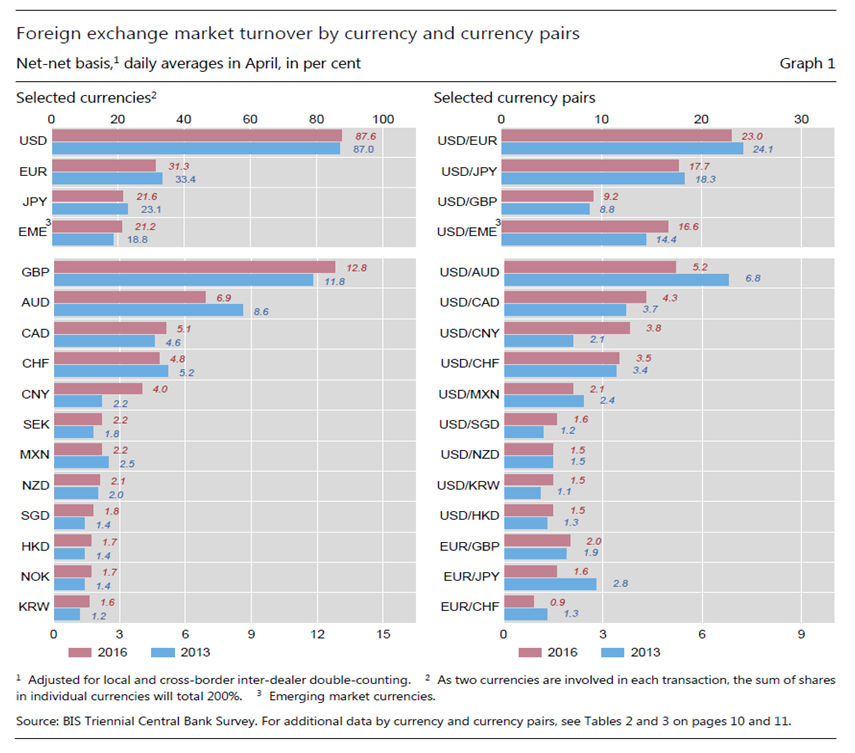 | Figure 1. Foreign Echange Market Turnover by Currency Pairs |
The figure 1 above summarizes the exchange rate relative to some selected currencies in the world market.
2. Review of Relevant Literature
So many Empirical econometric modeling works in Agricultural Economics, finance and economic data assume that relationships are linear. Economic theory plays a passive role on this issue, and thus most applied research finds it convenient to assume linearity. In the 2000's, some researchers try to challenge the empirical theory ―the random walk model predicts the exchange rate best‖. They used different methods and chose different models. For examples, data from Central and Eastern European countries was used to compare the forecasting models in transition economies [2]. Intraday foreign exchange rates were used as observations [9]. They found that some sophisticated time series models such as the Markov regime-switching model have better performance than the random walk models under the condition of intensive time period. Thus, the empirical theory ―the random walk model predicts the exchange rate best‖ does not work well sometimes. The thought expressed began to change based on irregularities observed in economic and financial data, that non-linear specifications is gradually becoming a more realistic representation of data generation processes. In finance, for instance, stock returns tend to be more correlated when there is low volatility than when volatility is high. A similar behavior has been observed in exchange rate mechanisms where the exchange rate may be constrained to lie within a pre-defined target zone [4]. To accommodate this kind of dynamic behavior using time series data, regime-switching models (RSM) have been introduced ([15] & [16]; [7]). Threshold autoregressive (TAR) model begins to be regularly appears in the agricultural economics literature as a model that is popularly used [18], and extensively discussed in Tong [17].
3. Mathematical Preliminaries of TAR and SETAR Models
3.1. SETAR Models
The SETAR model is a convenient way to specify a TAR model because qt is defined simply as the dependent variable  . In this case, the process can be formally written as
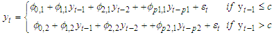 It is interesting to highlight that the estimation of SETAR models requires the application of least squares procedures only, more specifically, sequential conditional least squares. For the two-regime SETAR model, the steps can be outlined as follows:Step 1: Set
  for simplicity and estimate the AR coefficients conditional on the value of the threshold (c). Step 2: Calculate conditional residuals
  and estimated variances
  from the coefficients in step 1.Step 3: Obtain least squares estimates of c by minimizing the residual variance
  over all possible values of the threshold coefficient c, that is,
 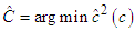 This minimization requires a direct search over the ordered values of
  [6] provides an approach free of nuisance parameters that are involved in estimation. Also note that in more complex models, the direct search may be over values of c and d, and thus, the estimate of the variance in Step 3 would be conditional on values of c and d (e.g., [6]). Step 4: Obtain final estimates of
  and
and  from results in Step 3.The estimation of the threshold values in Step 3 requires that each regime contains enough observations for reliable estimation of the AR coefficients. About fifteen percent (15%) of the observations on each regime seems to work well.
3.2. TAR Models
 If the above sequence is stationary, the least squares estimates of
  and
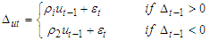
and  have an asymptotic multivariate normal distribution. The process is formally specified as:
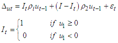
4. Description and Data Anaysis
The exchange rate data used in the study was extracted from Central Bank of Nigeria Bulletin of 2017. The data was obtained for 1996 to 2018.
4.1. Identification of a Stationary Condition of the Series
The line graph of the series Figure 2 indicates the non-stationarity of the series. There is evidence of volatility as the values do not fluctuate around a constant mean. The first differences of the series were taken (figure 3) and the graphs seem to fluctuate around a constant mean of zero value.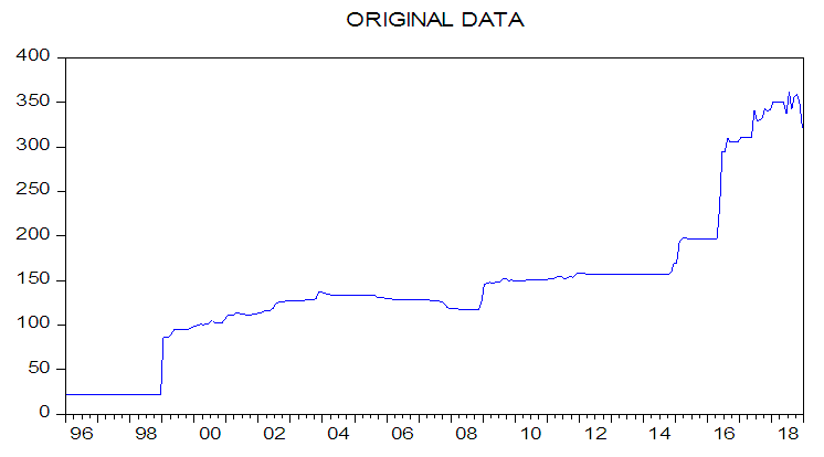 | Figure 2. Line Graph of the Leveled Exchange Rate of Naira/ Dollar |
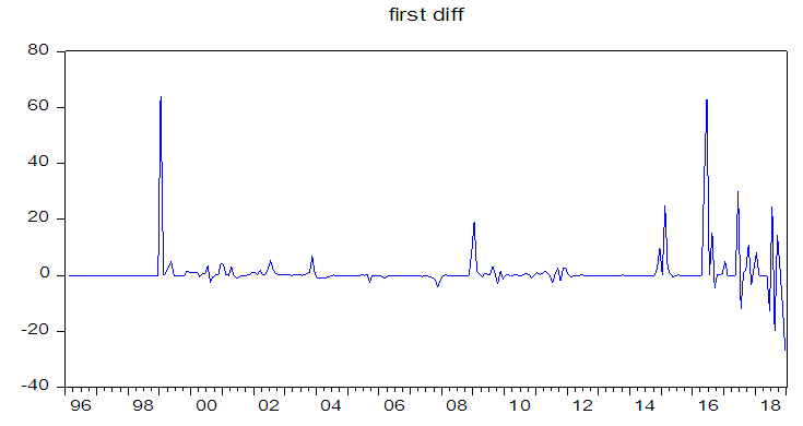 | Figure 3. Line Graph of the First Difference Exchange Rate of Naira/Dollar |
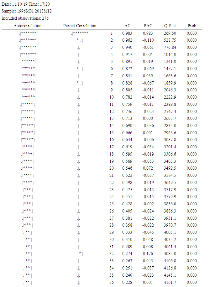
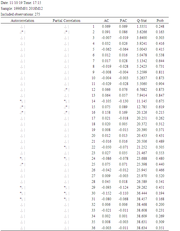
The results on the correlogram of the leveled for the series shows stronger evidence of non-stationarity since its autocorrelation coefficient function (ACF) of the residuals does not quickly decay to zero. On the other hand, the correlogram of the first difference shows that it is consistent with mean stationarity because most of the values promptly decay to zero. Tables 1 and 2 below show both the correlgrams for level and first difference.Table 1. Correlogram for Level
 |
| |
|
Table 2. Correlogram for First Difference
 |
| |
|
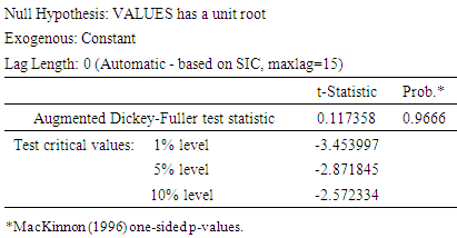
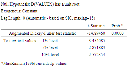
The stationary conditions of the series were formally verified by using Unit Root test (URT) for the leveled and first differences of the series. We tested for a unit root using the augmented Dickey-Fuller (ADF) statistic. At level, (table 3) all the series are not stationary but at first difference (table 4) all series appeared stationary as shown in the tables below:-Table 3. Original Data
 |
| |
|
Table 4. First Difference
 |
| |
|
4.2. Results of ARIMA Model Selection
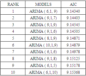
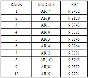
To identify the appropriate model parameter of ARIMA (p, d, q), AIC is adopted. From the unit root test, we obtain d to be 1. As to parameters p and q, we run the regression through the combinations of from p = 1 to p = 10 and from q = 1 to q = 10. For sake of saving space, we just list the top 10 with higher AIC values here. As shown in Table 5 below the model with the smallest value (9.14334) of AIC is the optimal ARIMA (6, 1, 9) chosen.Table 5. Arima Model Results
 |
| |
|
4.3. Results of SETAR Model
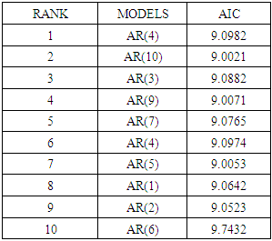
In our self-exciting threshold autoregressive (SETAR) model, we assume that a variable Naira is a linear autoregression within a regime. As there are two regimes in the study, the model could be written as SETAR (2, p, p). Panel A (table 6) is regime 1 of the two-regime SETAR and panel B (table 7) is regime 2. We select the most appropriate model by minimizing value of AIC. We build up a two-regime SETAR model, SETAR (2, 7, 4).Table 6. Panel A Regime 1 Observations Included 764
 |
| |
|
Table 7. Panel B Regime 2 Observations Included 308
 |
| |
|
4.4. Results Out-of-sample Forecasting Performance
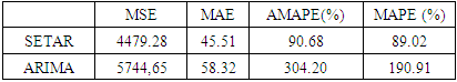
In this section, we check out-of-sample forecast performance of the two models. By checking multi-criteria (MSE, MAE, AMPE, and MAPE) on ARIMA and SETAR, we can compare the residual of these two models. For the mean squared error (MSE), SETAR is smaller than ARIMA with 4479.28 and 5744.65. This means SETAR has a fewer errors in the standard of MSE. For the mean absolute error (MAE), the adjusted mean absolute property error (AMAPE) and mean absolute property error (MAPE), SETAR is also smaller than ARIMA with fewer errors. According to our result shown in the table 8 below, the SETAR model is better than the ARIMA model over the sample period (second regime).Comparison of Forecasting Power.Table 8. Comarison of Forecasting Power by Models
 |
| |
|
5. Conclusions
At first, we believed there is no way for a linear regression to suit a series forever where stock prices follow a non-linear trend. Due to the economic environment changing, the stock market will be affected and change over time. Therefore, non-linear regression should be better than linear regression in the exchange rate market. First step of handling time series data is to check stationary state in the mean. We found out there was a unit root existed so we analyzed the first-difference. Next, we constructed an ARIMA model by using AIC selection criteria. And we build up a SETAR model by AIC as well. Afterward, we checked the forecasting power by four criteria (MSE, MAE, AMAPE, and MAPE) and all of those standards showed that SETAR has a stronger predicting power than ARIMA. The results also support previous assumptions of this thesis. Non-linear SETAR model is better than linear ARIMA model in Nigeria exchange rate market.
References
| [1] | Bank for International Settlements 2016. Triennial Central Bank Survey of Foreign Exchange and Derivatives Market Activity in April 2010: Preliminary Global Results. Bank for International Settlement, September. |
| [2] | Cuaresma, J. C., B. _Egert, & R. MacDonald (2005): \Non-linear exchangerate dynamics in target zones: A bumpy road towards a honeymoon."Working Paper 771, William Davidson Institute. |
| [3] | David, H., Lee, J., & Takizawa, H. (2010). In which exchange rate models do forecastters trust?: IMF Working Paper. |
| [4] | Franses, P. H. and D van Dijk. Non-linear time series models in empirical economics. NewYork, Cambridge University Press, 2000. |
| [5] | Hansen, B. E. (1996): “Inference when a Nuisance Parameter is not Identified under the Null Hypothesis,” Econometrica, 64, 413-430. |
| [6] | Hansen, B. E. (2000): “Sample Splitting and Threshold Estimation,” Econometrica, 68, 575-603. |
| [7] | Granger, C. W. J., and Terasvirta, T. (1993): Modeling Nonlinear Economic Relationships, Oxford, U.K. Oxford University Press. |
| [8] | Guha, B., & Bandyopadhyay, G. (2016). Gold Price Forecasting Using Arima Model. Journal of Advanced Management Science, Vol.4 (No.2). |
| [9] | Hong, Y. and Lee, T.H., (2003). Inference on predictability of foreign exchange rates via generalized spectrum and non-linear time series models. Review of Economics and Statistics, 85, 1048-1062. |
| [10] | Hongxing, L., Zhaoben, F., & Dongming, Z. (2007). GBP/USD Currency Exchange Rate Time Series Forecasting Using Regularized Least-Squares Regression Model. Proceeding of the World Congresson Engineering, Vol 2. |
| [11] | Isenah, G. M. O., Olusanya E. (2014). Forecasting Nigerian Stock Market Returns Using ARIMA and Artificial Neural Network Models. CBN Journal of Applied Statistics, Vol.5 (No.2). |
| [12] | Jarrett, J. E. K., Eric (2011). Arima modeling with intervention to forecast and analyze Chinese stock prices. International Journal of Engineering Business Management, Vol.3. |
| [13] | Meyler, A., Kenny, G., & Quinn, T. (1998). Forecasting Irish Inflation Using Arima Model (Vol. Vol. 1998, pp. 1-48): Ireland: Central Bank and Financial Services. |
| [14] | Mondal, P. S., Labani & Goswami, Saptarsi (2014). Study on Effectiveness of Time Series Modelling (Arima) in Forecasting Stock Prices. International Journal of Computer Science, Vol4 (No.2). |
| [15] | Priestly, E. (1980) “Using Threshold Cointegration to Estimate Asymmetric Price Transmission in the Swiss Pork Market,” Applied Economics: 679-87. |
| [16] | Priestly, E. (1988): “Threshold-Autoregressive, Median-Unbiased, and Cointegration Tests of Purchasing Power Parity,” International Journal of Forecasting, 14, 171-186. |
| [17] | Tong, H. (1990) Threshold Models in Non-Linear Time Series Analysis. New York: Springer Verlag. |
| [18] | Tong, H., & Lim, K. S. (1980). Threshold autoregressive, limit cycles and cyclical data. Journal of the Royal Statistical Society Series B, 42(3), 245–292. |
| [19] | Znaczko, T. M. (2013). Forecasting Foreign Exchange Rates. Applied Economics Theses, Vol.4. |

 Abstract
 Reference
 Full-Text PDF
 Full-text HTML