Edith U. Umeh, Chinyere I. Ojukwu
Department of Statistics, Nnamdi Azikiwe University, Awka, Nigeria
Correspondence to: Edith U. Umeh, Department of Statistics, Nnamdi Azikiwe University, Awka, Nigeria.
| Email: |  |
Copyright © 2019 The Author(s). Published by Scientific & Academic Publishing.
This work is licensed under the Creative Commons Attribution International License (CC BY).
http://creativecommons.org/licenses/by/4.0/

Abstract
This paper which discusses effects of influential outliers in local polynomial techniques (Kernel and Spline) aimed at determining the robust outliers where more than two independent variables are included in the model and to determine the best type of technique to be used for outlier treatment and its influence on the model performance. During the analysis, kernel and spline methods were applied on the Gross Domestic Product (GDP) of Nigeria, for the period of twelve years (1981 to 2012) from National Bureau of Statistics (NBS) using SPSS and Minitab to check whether outliers can be smoothed out during smoothing which was proved otherwise. Thus, three methods of outlier detection and elimination in local polynomial techniques namely Leverages, Mahalanobis distance and DFFITS were used to detect the influential outliers before smoothing. Seven outliers were detected from Mahalanobis distance with five high leverage cases and three influential outliers from DFFITS method. This inferential outliers affect the regression equation thereby deteriorate the model performance. It is therefore recommended that researchers carrying out research on smoothing techniques should detect and eliminate influential outliers before smoothing; hence the relevance of the effect of influential outliers in local polynomial techniques cannot be undermined.
Keywords:
Kernel smoother, Spline smoothing, Outlier, Leverage, Mahalanobis distance, Dffits
Cite this paper: Edith U. Umeh, Chinyere I. Ojukwu, Effects of Influential Outliers in Local Polynomial Techniques (Smoothing Techniques), International Journal of Probability and Statistics , Vol. 8 No. 1, 2019, pp. 19-22. doi: 10.5923/j.ijps.20190801.03.
1. Introduction
1.1. Background of the Study
Smoothing by local fitting is actually an old idea that is deeply buried in the methodology of time series, where data measured at equally spaced points in time were smoothed by local fitting of polynomial methods into more general case of regression analysis, Fan and Gijbels (1996). In statistics, polynomial regression is a form of linear regression in which the relationship between the independent variable x and the dependent variable y is modelled as an nth degree polynomial. It fits a non-linear relationship between the value of x and the corresponding conditional mean of y, denoted by E(y/x). The regression function E(y/x) is linear in the unknown parameters that are estimated from the data; for this reason, polynomial regression is considered to be special case of multiple linear regression. Nonetheless, it may be convenient not to force data into models but just to attempt to moderate frantic data by using a classic and straight-forward statistical approach known as data smoothing. There are several ways to achieve data smoothing, especially through statistical techniques: among these approaches based on regression analysis are kernel method, local regression, spline methods and orthogonal series.Kernel Regression is a non-parametric technique in statistics used to estimate the conditional expectation of a random variable. The idea of kernel regression is putting a set of identical weighted function called a kernel function to each observational data point. The kernel estimate is sometimes called the Nadaraya-Watson estimate; More discussion of this and other weaknesses of the kernel smoothers can be found in Hastie and loader (1993). Local regression is an approach to fitting curves and surfaces to data in which a smooth function may be well approximated by a low degree polynomial in the neighbourhood of point (Loader, 2012). To use local regression in practice, we must choose the bandwidth, the parametric family and the fitting criterion. Local regression has many strengths including correction of boundary bias in kernel regression. Singly, none of these provides a strong reason to favour local regression over other smoothing methods such as smoothing spline and orthogonal series. Smoothing spline is another popular and established nonparametric regression, which is based on spline as a natural, coherent and modern approach to outliers on the optimization of a penalized least square criterion whose solution is a piecewise polynomial or spline function. This approach employs fitting a spline with knots at every data point, so it could potentially fit perfectly into data, but the function parameters are estimated by minimizing the usual sum of square criterion (Garcia, 2010). Orthogonal series methods represent the data with respect to a series of frequency terms of orthogonal basis functions, such as Sines and Cosines. Only the low frequency trems are retained Efromovich (1999) provides a detailed discussion of this approach to smoothing. A limitation of orthogonal series approaches is that they are more difficult to apply when the xi are not equally spaced and there is no relationship between the explanatory variables and the responding variables. Each of the smoothing methods discussed above has one or more’’ smoothing parameter’’ that controls the amount of smoothing being performed.In all these smoothing methods none of them has considered outlier detection and treatment. The common practice is to treat outliers at the beginning of the analysis and then proceed with no additional thought given to the outliers. They see outliers as extreme observations, the points that lie far beyond the scatter of the remaining residuals in a residual plot. i.e. observations which are well separated from the remainder of the data. These outlying observations may involve large residuals and often have dramatic effects on the fitted regression function. Ruppert and Wand (1994) studied bias and variance; their result cover arbitrary degree local polynomial and multidimensional fits for bias and the term depending on the weight function varies according to the degree of local polynomial, generally increases as the degree of the polynomials increases for variance. They also discuss the local linear estimator, nobody has previously developed an improved estimator using the information of outliers. Cleveland and Devlin (1988) researched on the degree of freedom under the different methods and found out that the degree of freedom provides a mechanism by which different smoothers, with different smoothing parameter, can be compared. They simply choose smoothing parameters producing the same number of degrees of freedom; in all these, no attention has been given to improve estimators using the information of outliers. Thus the need for this paper which used Leverages, Mahalanobis distance and DFFITS methods of outlier detection/elimination on kernel and Spline smoothing techniques to check whether it will have effects on the model performance. Gross Domestic Product (GDP) of Nigeria from 1981 to 2012 was used for the analysis.
2. Methods
2.1. Kernel Smoother (KS)
The basic idea of kernel smoothing is to estimate the density function at a point  using neighbouring observations. A usual choice for the kernel weight w is a function that satisfies
 | (1) |
With joint pdf | (2) |
The estimate of  is called the kernel density estimator. Nadaraya Watson estimator of the conditional moment is
 | (3) |
Where h is the bandwidth which determines the degree of smoothness and w is symmetric kernel function.
2.2. Smoothing Spline
Hardle, (1991) researched on a seemingly very different set of smoothing techniques called the smoothing spline. An entirely different approach to smoothing is through optimization of a penalized least square criterion, thus | (4) |
Where  is a smoothing parameter which plays the same role as the bandwidth in kernel smoothing.The first term in equation (4) which is PLS
  residual sum of squares.The second term
  is a roughness penalty, which is large when the integrated second derivation of the regression function
  is large; that is, when
  is “rough” (with rapidly changing slope).
2.3. Leverages 
The leverage score for the  data unit is defined as
 | (5) |
which is the  diagonal element of the projection matrix
 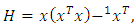 | (6) |
where X is the design matrix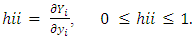 | (7) |
where  and
and  are the fitted and measured observations respectively. The diagonal elements
  have some useful properties.
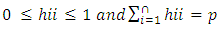 | (8) |
where P is the number of regression parameters in the regression function including the intercept term. The diagonal elements  in the hat matrix is called the leverage (in terms of the x values) of the
  observation.
2.4. Mahalanobis Distance
Let X be an n x p matrix representing a random sample of size n from a p- dimensional population. Mahalanobis distance (MDi) of the  observation defined as
  | (9) |
is the Mahalanobis distance of point  (Mahalanobis, 1936).A decision criterion can be chosen since the MDi (Mahalanobis distance) follows a
  distance with p degrees of freedom.E.g.
 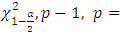 degree of freedom will be minus one if the independent variables is more than 2 at
  significance level.MD1 measures the distance of each data point from the centre of mass of the data point based on covariance and variances of each variables. The cut-off points is usually taken at the 97.5th percentile of
  distribution. Any observation with MDi values greater than the cut-off point, may give an indication of outlyingness.Rousseeuw and Leroy (1987) suggested a cut-off point for RMDi (Robust Mahalanobis distance) as
 This is the same cut-off point as MDi, where any value greater than the cut-off point may be declared as outliers. This cut-off value comes from the assumption that the p-dimensional variables follow a multivariate normal distribution.
2.5. Difference in Fits (DFFITS)
Studentization is achieved by dividing the estimated standard deviation of the fit at that point.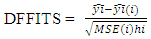 | (10) |
Where  is the prediction for point i with and without point i included in the regression, MSE (i) is the Mean standard error estimated without the point in question and
  is the leverage for the point and is calculated by deleting the ith observation.Large values of /DFFITS/ indicate influential observations. A general cut-off to consider is 2, a size adjusted cut-off recommended by Belsley, kuh, and welsch (1980) is
  where n is the number of observations used to fit the model and p is the number of parameters in the model.
3. Results
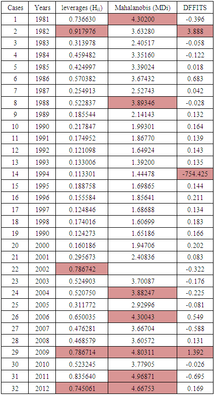
Table 1. Table Showing the Leverages, Mahalanobis Distance and DFFITS of the Nigerian GDP Data from 1981-2012
 |
| |
|
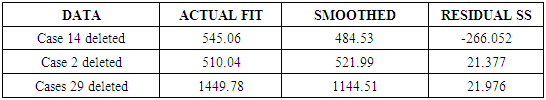
Table 2. Table Showing the Deleted Cases of High Influential Outliers
 |
| |
|
4. Discussion
From Table 1 above seven outliers (cases 1, 8, 24, 26, 29, 31, 32) have Mahalanobis distance of 4.30, 3.89, 3.88, 4.80, 4.97 and 4.67 representing years 1981, 1988, 2004, 2006, 2009, 2011, 2012 respectively. They are the only items exceeding the critical value of  from the chi- square distribution table.A leverages > 2(p/n) =0.75 and very isolated is an outlier but may or may not actually be influential because leverages only take into account the extremeness of the X values. Four high leverages (cases 2, 22, 29, 32) with points 0.92, 0.79, 0.79, 0.75 representing years 1982, 2002, 2009, 2012 respectively have high leverages above the critical value of 2(p/n)./DFFITS/ indicated cases 2, 14, and 29 as influential outliers with points 3.89, 754.425 and 1.39 respectively which is greater than the critical value of
  .From Table 2 above, it is clear that case 14 is very influential, but cases 2 and 29 are not relatively influential to case 14 though their values are larger than the reference values. Case 14 is also very influential on the kernel smooth and spline smooth. If we remove case 14, the kernel smooth and spline smooth reduces from 545.06 to 484.53 and the form of the fitted curve changes from almost linear to cubic.Therefore, in the existence of influential outlier from the results of the analysis, the mahalanobis distance produces multiple outliers that may not be influential which may lead to invalid inferential statements and inaccurate predictions. In this situation DFFITS estimator is recommended because it gives more efficient estimates of influential points. This is the reason why it is important to identify influential outliers as they are responsible for the misleading inferences about the fitting of the regression model. By correctly detecting those observations, may help statistical methods to analyze their data. The overall results from Table 1 indicate that mahalanobis distance is not efficient enough because it suffers from masking effects while DFFITS tend to swamp few low leverage points. Nevertheless, the swamping rate of mahalanobis distance is less than the DFFITS. The numerical examples signify that the DFFITS offers a substantial improvement over the other existing methods. The DFFITS successfully identifies high influential points with the lowest rate of swamping.
References
| [1] | Avery, M. (2012), Literature Review for local polynomial regression. http://www4.ncsc.edu/mravery/AveryReview2.pdf, Accessed 20/05/2015. |
| [2] | Davies, L., Gather, U (1993). “The identification of multiple outliers’’, Journal of the American statistical Association, 88(423), 782-792. |
| [3] | Fan J. & Gijbels I. (1996). Local polynomial modeling and its applications, Chapman and Hall. |
| [4] | Fung, W. (1993), “Unmasking outliers and leverage points’’, A confirmation. Journal of the American Statistical Association, 88, 515-519. |
| [5] | Grubbs, F.E. (1969), “Procedures for detecting outlying observations in samples,’’ Technometrics, 11, 1-21. |
| [6] | Hadi, A.S. (1992), Identifying multiple outliers in multivariate Data. Journal of the royal statistical society B, 54, 761-771. |
| [7] | Hawkins, D.. (1980), “Identification of outliers,’’ Chapman and Hall, London. |
| [8] | Imon A.H.M.R (2002), “Identifying multiple high leverage points in linear regression,’’ Journal of Applied statistics, 32, 929-946. |
| [9] | Dursun A. (2007). A Comparison of the nonparametric regression models using smoothing spline and kernel regression. International journal of mathematical, computational, physical, Electrical and computer Engineering 1(12). |
| [10] | Mahalanobis, P.C (1936). On the generalized distance in statistics PDF .Proceedings of the national institute of science of india. 2(1): 49-55. |
| [11] | Meloun M & Militky J.. (2001). Detection of single influential points in OLS. Regression model building. AnalyticachimicaActa, 439, 169-191. |
| [12] | Nadaraya, E.A (1964). On estimating regression, (Theory of probability and its applications), 9: 141-142 |
| [13] | Nugent, Pam M.S (2013), “DFFITS’’, Psychology dictionary.org. Professional Reference. |
| [14] | Rousseeuw P.J, & Leroy A.M. (1987). Robust regression and outlier detection. John Wiley and sons, Inc. New York, USA. |
| [15] | Rousseeuw P.J, & Van Zomeren B.C. (1990), “Unmasking multivariate outliers and leverage points,’’ Journal of the American statistical Association, 85(411), 633-651. |
| [16] | Simonoff, J.S, (1996), Smoothing methods in statistics. Springer New York. |
| [17] | Thompson G.L (2006). An SPSS implementation of the no recursive outlier detection procedure with shifting Z score criterion. Behavior Research Methods, 38, 344-352. |
| [18] | Wahba, G.. (1990). Spline model for observational data. SIAM (society for industrial and applied mathematics), Philadelphia. |
| [19] | Wand, M.P & Jones M.C, (1995), Kernel Smoothing. London: Chapman and Hall. |
| [20] | Www.mathsisfun.con/estimate. |
| [21] | Www.merriam-webster.com/analysis. |
| [22] | Www.Wikipedia 2016. |

 Abstract
 Reference
 Full-Text PDF
 Full-text HTML