Ogunleye L. I.1, Oyejola B. A.2, Obisesan K. O.3
1Business Process Reengineering, Guaranty Trust Bank Plc. Plot 1400, Tiamiyu Savage Street, Lagos, Nigeria
2Department of Statistics, University of Ilorin, Ilorin, Nigeria
3Department of Statistics, University of Ibadan, Ibadan, Nigeria
Correspondence to: Ogunleye L. I., Business Process Reengineering, Guaranty Trust Bank Plc. Plot 1400, Tiamiyu Savage Street, Lagos, Nigeria.
| Email: |  |
Copyright © 2018 The Author(s). Published by Scientific & Academic Publishing.
This work is licensed under the Creative Commons Attribution International License (CC BY).
http://creativecommons.org/licenses/by/4.0/

Abstract
The normal distribution is the bedrock of many statistical procedures. Inferences and conclusions from parametric statistical analysis may not be valid when the normality assumption is violated. Three common procedures used for evaluating whether a random sample of independent observations come from a population with normal distribution are: graphical methods (histograms, box plots, Q-Q-plots), numerical methods (skewness and kurtosis) and formal normality tests. In this study, the type I error rates and power of four common formal tests of normality: Anderson-Darling (AD) test, Chi-square (CS) test, Kolmogorov-Smirnov (KS) test and Shapiro-Wilk (SW) test were compared. Type I error rate of the four tests were computed via simulation (in R) of sample data generated from the standard normal while power comparisons was conducted using common continuous and discrete type as well as less common mixture normal alternative distributions. Five thousand independent samples of various sample sizes were generated from the different distributions considered. Our findings reveal that Shapiro-Wilk test has the most acceptable type I error rate amongst the four tests, followed by Kolmogorov-Smirnov test, Anderson-Darling test and Chi-square test. The power study revealed that none of the four tests is uniformly most powerful for all types of alternative distributions under consideration. Shapiro-Wilk test is the most powerful amongst the four normality tests for continuous –type alternative distributions while Chi-square test outperforms the other three tests for discrete-type distributions. All four normality tests have significantly low powers under the mixture normal distributions with unequal means and equal variances irrespective of the mixture probabilities while there is an improved performance under mixture normals with unequal means and unequal variances.
Keywords:
Simulation, Normality tests, Mixture Normal, Type I error rates, Power of test
Cite this paper: Ogunleye L. I., Oyejola B. A., Obisesan K. O., Comparison of Some Common Tests for Normality, International Journal of Probability and Statistics , Vol. 7 No. 5, 2018, pp. 130-137. doi: 10.5923/j.ijps.20180705.02.
1. Introduction
According to Thode (2002), “normality is one of the most common assumptions made in the development and use of statistical procedures.” The dependence of most parametric statistical methods on the normality assumption shows the importance of normality tests in statistical analysis. Inferences from parametric statistical analysis may not be valid when the normality assumption is violated. Therefore, before embarking on any statistical analysis, it is important to test the normality assumption. The easiest way to assess normality is by using graphical methods. The normal quantile-quantile plot (Q-Q plot) is one of the most effective and commonly used diagnostic tool for checking normality of data. Even though the graphical methods are useful tool in assessing normality, they do not provide not sufficient conclusive evidence that the normality assumption holds. Therefore, to support the graphical methods, formal procedures namely numerical methods and normality tests should be performed before passing any judgement about the normality of the data.The numerical methods include skewness and kurtosis coefficients whereas normality test is a more formal hypothesis testing procedure to ascertain if a particular data follows a normal distribution or not. Significant number of normality tests are available in literature, however, the most common normality test procedures available in statistical software packages are the Anderson-Darling (AD) test, Chi-square (CS) test, Jarque-Bera (JB) test, Kolmogorov-Smirnov (KS) test, Lilliefors test and Shapiro-Wilk (SW) test. The different tests of normality often generate different outputs i.e. some tests reject while others accept the same the null hypothesis of normality for the same dataset. These conflicting results could be misleading and often confusing. Therefore, the choice of test of normality to be used under different circumstance should be given significant attention. Consequently, this study seeks to explain the behaviours of four normality tests under selected discrete and continuous distributions.
2. Methodology
TYPE I ERROR RATE and POWERThe most important property of a test is that it guarantees that the rate of erroneously rejecting the null hypothesis will not be too high. Otherwise, we would reject H0 too often when in fact the sample comes from a normal population.The test decision of rejecting the null hypothesis when it is actually true is called type I error. The probability of making a type I error is denoted α and often called the significance level of a test.We performed empirical studies based on simulations. The underlying principle is described as follows:If N is the number of randomly generated independent samples of size n where all N samples follow a standard normal distribution, the empirical type I error rate αn,N of a given test for a given sample size n is given by  Where r is the number of times the null hypothesis is rejected in N tests. The objective is to check for a given test of normality if αn is higher or lower than α.The test decision of not rejecting the null hypothesis H0 when the alternative hypothesis H1 is true is called type II error and is denoted by β. The power of a statistical test (1- β) is the probability of making the right decision i.e. rejecting a null hypothesis when it is not true. Let N be the number of randomly generated independent samples of sizes n, where all N samples follow the same distribution that is non-normal. The empirical power
  of a given test for normality for a given significance level α is given by
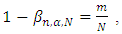 Where m ≤ N is the number of the m tests that reject the null hypothesis of a normally distributed sample at the significance level α.In this study, simulation procedure was used to evaluate the empirical power of AD, CS, KS and SW test statistics in testing if a random sample of n independent observations come from a population with normal
  distribution. The null and alternative hypotheses are:
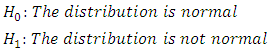 Three levels of significance α = 1%, 5% and 10% were considered to investigate the effect of the significance level on the power of the tests. In order to obtain the simulated power of the four of the four normality tests, the setting for the simulation parameters were the same as in the empirical type II error investigations.VALUES OF PARAMETERS USED IN THE STUDYn = 10, 20, 30, 40, 50, 100, 200, 300, 400, 500, 1000N = 5000α = 0.01, 0.05 and 0.10Normality Tests: Anderson-Darling (AD), Chi-square (CS), Kolmogorov-Smirnov (KS), and Shapiro-Wilk (SW)The alternative distributions were selected to cover both continuous and discrete probability distributions. The alternative distributions considered were three continuous distributions; U (0, 1), Beta (2, 2), Gamma (4, 5) and two discrete distributions; Binomial (n, 0.5) and Poisson (4).
3. Results & Discussion
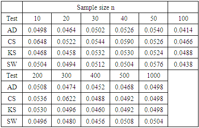
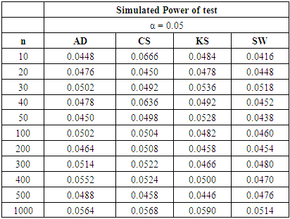
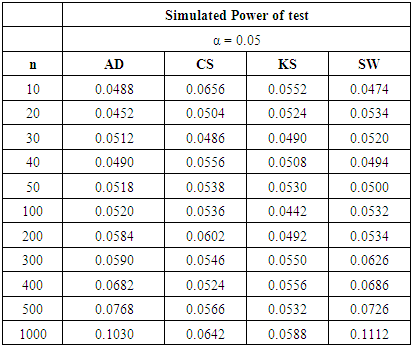
Table 1 shows the result of the rate at which each of the four normality tests reject a true null hypothesis.
3.1. Type I Error
Table 1. Empirical type I error rate for each test and given sample size
 |
| |
|
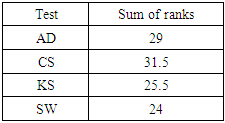
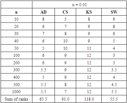
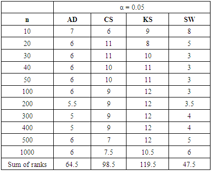
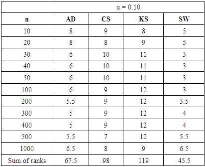
In order to compare the performance of the different normality tests, the ranking procedure was applied. Rank 1 was assigned to the test whose type I error rate is closest to 0.05 while rank 4 was given to the test that is least close to 0.05. The ranking was done for each sample size and the sum of ranks for each test was obtained. The test with the lowest sum of rank is considered as the best test among those in our collection. Table 2 shows the sum of ranks across all sample sizes for each test.Table 2. Sum of ranks based on type I error rates for each normality test
 |
| |
|
Table 2 shows that the Shapiro-Wilk test is the best among the four normality tests because it has the lowest sum of ranks. It is closely followed by the Kolmogorov-Smirnov test and the Anderson-Darling test. Chi-square goodness-of-fit test has the largest sum of ranks and hence the poorest.The type I error rate of each of the four tests does not show any consistent pattern with changes in the sample size.
3.2. Power of the Tests
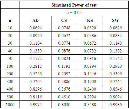
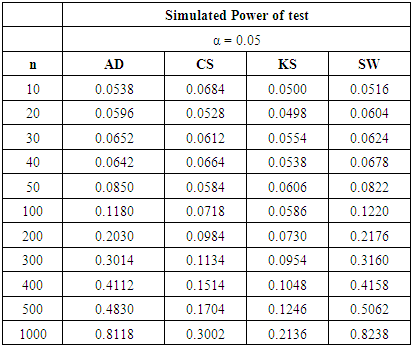
3.2.1. Power for Continuous Alternative non-normal Distributions
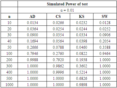
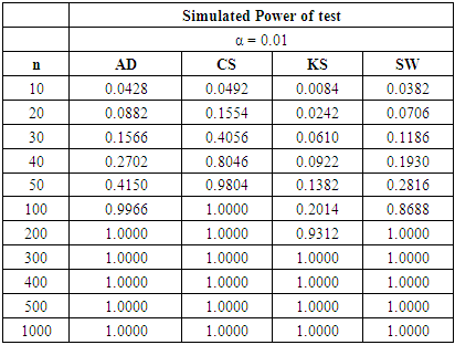
The following tables show that the power of the tests varies with the significance levels, sample sizes and three different continuous alternative distributions. The tables show the power for selected alternative distributions for α = 0.01, 0.05 and 0.10.Table 3. Power Comparison for Different Normality Tests against U (0, 1) alternative distribution at α = 0.01
 |
| |
|
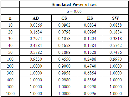
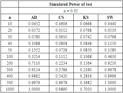
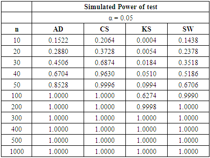
Table 4. Power Comparison for Different Normality Tests against U (0, 1) alternative distribution at α = 0.05
 |
| |
|
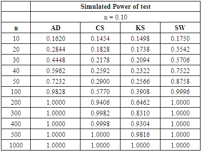
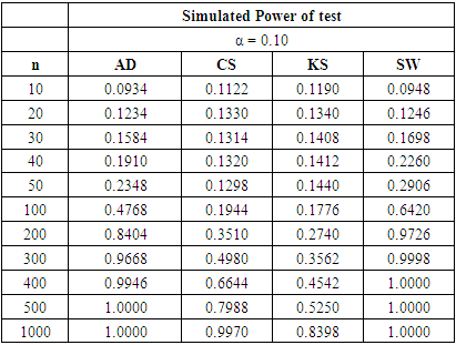
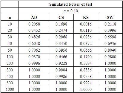
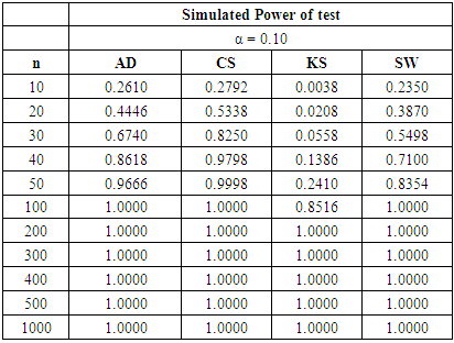
Table 5. Power Comparison for Different Normality Tests against U (0, 1) alternative distribution at α = 0.10
 |
| |
|
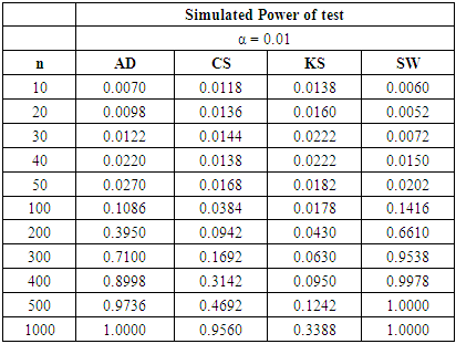
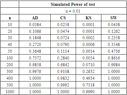
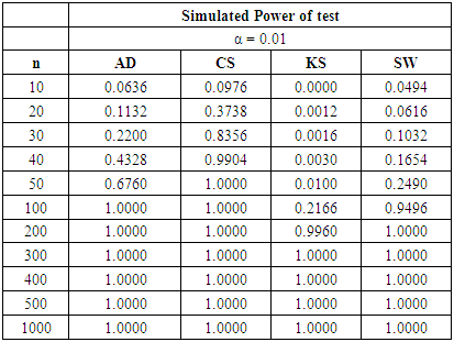
Table 6. Power Comparison for Different Normality Tests against Beta (2, 2) alternative distribution at α = 0.01
 |
| |
|
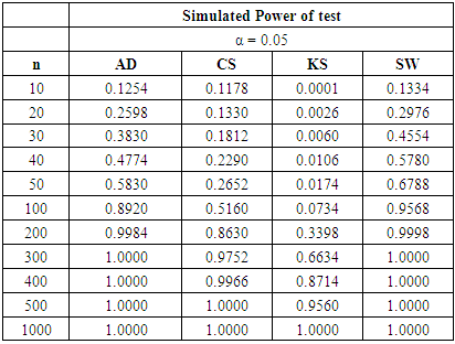
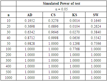
Table 7. Power Comparison for Different Normality Tests against Beta (2, 2) alternative distribution at α = 0.05
 |
| |
|
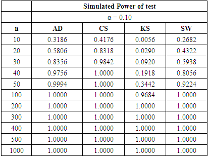
Table 8. Power Comparison for Different Normality Tests against Beta (2, 2) alternative distribution at α = 0.10
 |
| |
|
For all significance levels considered, the four tests showed very low power values at samples sizes between 10 and 50 inclusive. None of these tests produced power value of 40% at n = 10, 20, 30, 40 and 50. The SW test performed as the most powerful at these sample sizes. At α = 0.10 and a pre-determined power of 80%, the SW test requires n > 200 to attain the desired power while a sample size of n > 300 is needed by the AD test be 80% powerful. The CS test will require a sample size that is significantly greater than 500 before it can attain 80% power while a sample size of 1,000 is not large enough for the KS test to attain 80% power.Tables 6, 7, and 8 above showed that the power behaviours of the four normality tests is different from what we observed under the U (0, 1) alternative distribution. For all significance levels considered, the four tests showed very low power values at samples sizes between 10 and 50 inclusive. None of the tests produced power value of 40% at n = 10 to 50 and the SW test is still the most powerful at these sample sizes.At α = 0.01 and a pre-determined power of 80%, the SW test requires n > 200 to attain the desired power while a sample size of n > 300 is required by the AD test be 80% powerful. The CS test will require a sample size that is significantly greater than 500 before it can attain 80% power while a sample size as large as 1000 is not large enough for the KS test to be 80% powerful.For α = 0.05 and a pre-specified power of 80%, the sample sizes required by individual test reduced compared to α = 0.01. The SW test will require n > 100 while a sample size between 200 and 300 will make the AD test 80% powerful. The CS test requires sample size more than 500 to attain 80% power while the KS could not attain this power value even at n= 1000. When α is increased to 0.10, the KS test attain a power value of 83.98% at  whereas the other tests required lower sample sizes for the desired power.The four normality tests showed improved power behaviours under the gamma alternative distribution in tables 6, 7 and 8 above. The least powerful KS test in our collection even showed acceptable power values though not comparable to the other three. The power of the SW test at sample size n = 50 for all significance levels considered is greater than 40%. The AD test also showed improved power for these small sample sizes particularly at α = 0.05 and 0.10 respectively.
Table 9. Power Comparison for Different Normality Tests against Gamma (4, 5) alternative distribution at α = 0.01
 |
| |
|
Table 10. Power Comparison for Different Normality Tests against Gamma (4, 5) alternative distribution at α = 0.05
 |
| |
|
Table 11. Power Comparison for Different Normality Tests against Gamma (4, 5) alternative distribution at α = 0.10
 |
| |
|
At α = 0.05 level of significance, the SW test requires a sample size slightly higher than 50 to yield 80% power value. The sample size requirement of the AD test is similar to that of the SW test. The CS test will require sample size n > 100 to be 80% powerful. The KS test still requires the highest sample size to attain a comparable pre-specified power.
3.2.2. Power for Discrete Alternative Non-normal Distributions
The following tables show that the power of the tests varies with the significance levels, sample sizes and three different discrete alternative distributions. The tables show the power for selected alternative distributions for α = 0.01, 0.05 and 0.10.Tables 12, 13, and 14 below show that the CS test is the most powerful of the four test for all significance levels considered. At α = 0.01 and n = 30, the power of the CS test is even more than our desired 80%. To obtain a pre-specified 80% power, the AD test will require a sample size lower than what will be required by the SW test in the range of n > 60. The KS test still require the highest sample size of n > 100 to be 80% powerful. As α increases, the sample size requirements for a desired power value of each test decreases.Table 12. Power Comparison for Different Normality Tests against Binomial (n, 0.5) alternative distribution at α = 0.01
 |
| |
|
Table 13. Power Comparison for Different Normality Tests against Binomial (n, 0.5) alternative distribution at α = 0.05
 |
| |
|
Table 14. Power Comparison for Different Normality Tests against Binomial (n, 0.5) alternative distribution at α = 0.10
 |
| |
|
Table 15. Power Comparison for Different Normality Tests against Poisson (4) alternative distribution at α = 0.01
 |
| |
|
Table 16. Power Comparison for Different Normality Tests against Poisson (4) alternative distribution at α = 0.05
 |
| |
|
Table 17. Power Comparison for Different Normality Tests against Poisson (4) alternative distribution at α = 0.10
 |
| |
|
Tables 15, 16 and 17 show a fall in the power value of the four tests when compared with the binomial alternative distribution. We also observed that the CS test is still the most powerful across all sample sizes and significance levels considered amongst the four tests. The AD test has a comparable power with the CS test while the KS is the least powerful in this collection. The sample size required by the CS to attain a desired power under the discrete distributions considered is lower than what was required for the three continuous alternative distributions earlier simulated.
3.2.3. Power of Tests for Mixture Distributions
Here, we considered the following mixture of two normal distributions:i. Unequal means and equal variance with equal probabilities of mixture denoted Mixture Normal 1 as {N1 (-1, 4) + N2 (1, 4), p1 = p2 = 0.5}ii. Unequal means and equal variance with unequal probabilities of mixture denoted Mixture Normal 2 as {N1 (-1, 4) + N2 (1, 4), p1 = 0.3 & p2 = 0.7}iii. Unequal mean and unequal variance with equal probabilities of mixture denoted Mixture Normal 3 as {N1 (-1, 2) + N2 (1, 4), p1 = p2 = 0.5} iv. Unequal mean and unequal variance with unequal probabilities of mixture denoted Mixture Normal 4 as {N1 (-1, 2) + N2 (1, 4), p1 = 0.3 & p2 = 0.7}Where p1 & p2 are the mixture probabilities for the two normal distributions respectively.The ranking procedure was adopted to obtain a clearer picture of the performance of the different normality tests. The rank 1 was given to the test with the highest power while rank 4 was assigned to the test which has the lowest power. The ranks were then summed to obtain the grand total of the ranks. Since the lowest rank was given to the test with the highest power, therefore the test which has the lowest sum of rank will be chosen as the most powerful test in our collection in detecting departure from normality. The following tables show the rank of power based on the type of alternative distribution and sample sizes, respectively.Table 18. Power Comparison against Mixture Normal 1 at α = 0.05
 |
| |
|
Table 19. Power Comparison against Mixture Normal 2 at α = 0.05
 |
| |
|
Table 20. Power Comparison against Mixture Normal 3 at α = 0.05
 |
| |
|
Table 21. Power Comparison against Mixture Normal 4 at α = 0.05
 |
| |
|
Table 22. Rank of Power of tests under all three continuous alternative distributions at α = 0.01
 |
| |
|
Table 23. Rank of Power of tests under all three continuous alternative distributions at α = 0.05
 |
| |
|
Table 24. Rank of Power of tests under all three continuous alternative distributions at α = 0.10
 |
| |
|
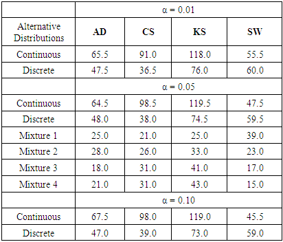
Table 25. Total Rank of Power based on the type of Alternative distribution
 |
| |
|
In summary, the sums ranks of power of the four tests under the continuous, discrete distributions and mixture normals are presented.Power analysis show that the choice of a normality test should be made with special consideration for the type of measurement in which the observed data are collected. Under the three continuous alternative distribution considered in this study, Shapiro-Wilk test is the most powerful test amongst the four tests for all significance levels considered. The Anderson-Darling test may also be adopted in place of the Shapiro-Wilk test due to its reasonable power comparison against the Shapiro-Wilk test. Chi-square test and Kolmogorov-Smirnov test have low power for the continuous alternative distributions considered.Chi-square test is the most powerful of the four tests under the two discrete alternative distributions considered. It consistently demonstrated the highest power for all significance levels considered. The Anderson-Darling test again is next to the Chi-square test, followed by Shapiro-Wilk test. The Kolmogorov-Smirnov test is the least powerful among the four normality tests considered in this work.The power of all four tests, regardless of the two mixture probabilities considered, were very low under the mixture of two normal distributions with unequal means and equal variance. However, with a mixture probability of 0.5 each, Shapiro-Wilk test out-performed the other three tests under mixture of two normals with unequal means and unequal variances. This is closely followed by the Anderson-Darling test, then the Chi-Square and Kolmogorov Smirnov tests respectively.We also found that the power of the four tests generally increase as the sample size and significance level increase as expected theoretically.
4. Conclusions
None of the four tests considered in this study is uniformly most powerful for all types of distributions, sample sizes and significance levels considered.For continuous alternative distributions, Shapiro-Wilk test is the most powerful test for all sample sizes whereas Kolmogorov-Smirnov test is the least powerful test in our collection. However, the power of Shapiro-Wilk test is still low for small sample size. The performance of Anderson-Darling test is quite comparable with Shapiro-Wilk test.For discrete alternative distributions, Chi-square test outperforms the other three tests at all sample sizes. Anderson-Darling test is next to it while Shapiro-Wilk test performs better than Kolmogorov-Smirnov test.Given the inconsistencies in power performance of all four tests under mixture of two normal distributions, we recommend that more work should be carried out on the search for normality tests which will perform better under these special conditions and the effect of mixture probabilities on the performance of normality tests.
References
| [1] | Althouse, L.A., Ware, W.B. and Ferron, J.M. (1998). Detecting Departures from Normality: A Monte Carlo Simulation of a New Omnibus Test based on Moments. |
| [2] | Anderson, T.W. and Darling, D.A. (1954). A Test of Goodness of Fit. Journal of the American Statistical Association, Vol. 49, No. 268, 765-769. |
| [3] | Arshad, M., Rasool, M.T. and Ahmad, M.I. (2003). Anderson Darling and Modified Anderson Darling Test for Generalized Pareto Distribution. Pakistan Journal of Applied Sciences 3(2), pp. 85-88. |
| [4] | Conover, W.J. (1999). Practical Nonparametric Statistics. Third Edition, John Wiley & Sons, Inc. New York, pp. 428-433 (6.1). |
| [5] | D’Agostino, R. and Pearson, E.S. (1973). Test for Departures from Normality. Empirical Results for the Distribution of  . Biometrika, Vol.60, No. 3, pp.613-622. . Biometrika, Vol.60, No. 3, pp.613-622. |
| [6] | D’Agostino, R.B. and Stephens, M.A. (1986). Goodness-of-fit Techniques, New York: Marcel Dekker. |
| [7] | Dufour J.M., Farhat, A., Gardiol, L. and Khalaf, L. (1998). Simulation-based Finite Sample Normality Tests in Linear Regression. Econometrics Journal, Vol.1, pp.154-173. |
| [8] | Farrel, P.J. and Stewart, K.R. (2006). Comprehensive Study of Tests for Normality and Symmetry: Extending The Spiegelhalter Test. Journal of Statistical Computation and Simulation, Vol. 76, No. 9, pp. 803-816. |
| [9] | Jarque, C.M. and Bera, A.K. (1987). A test for normality of observations and regression residuals, Internat. Statst. Rev. 55(2), pp.163-172. |
| [10] | Kolmogorov, A.N. (1933). Sulla determinazioneempirica di unalegge di distribuzione, Giornaledell’ Instituto Italianodegli Attuari 4, pp. 83-91 (6.1). |
| [11] | Lilliefors, H.W. (1967). On the Kolmogorov-Smirnov Test for Normality with Mean and Variance Unknown. Journal of American Statistical Association. Vol. 62, No. 318, pp. 399-402. |
| [12] | Mendes, M. and Pala, A. (2003). Type I error Rate and Power of Three Normality Tests. Pakistan Journal of Information and Technology 2(2), pp. 135-139. |
| [13] | Normadiah, M.R. and Yap, B.W. (2010). Power Comparisons of some selected normality tests. Proceedings of the Regional Conference on Statistical Sciences, pp. 126-138. |
| [14] | Park, H.M. (2008). Univariate Analysis and Normality Test Using SAS, Stata, and SPSS. Technical Working Paper. The University Information Technology Services (UITS) Center for Statistical and Mathematical Computing, Indiana University. |
| [15] | Royston, P. (1992). Approximating the Shapiro-Wilk W test for Normality [Abstract]. Statistics and Computing, 2, pp.117-119. |
| [16] | Seier, E. (2002). Comparison of Tests for Univariate Normality. InterStat Statistical Journal, 1, pp.1-17. |
| [17] | Shapiro, S.S. and Wilk, M.B. (1965). An Analysis of Variance Test for Normality (Complete Samples). Biometrika, Vol. 52, No. 3, pp. 591-611. |
| [18] | Thadewald, T. and Buning, H. (2007). Jarque-Bera and its Competitors for Testing for Normality. Journal of Applied Statistics, Vol. 34, No.1, pp. 87-105. |
| [19] | Thode, H.C. Testing for Normality. Marcel Dekker, New York, 2002. |

 Abstract
 Reference
 Full-Text PDF
 Full-text HTML