1. Introduction

Longitudinal studies are very common in many fields such as medicine, public health, psychology, biology and more. In the simplest design of univariate longitudinal data a single response is collected repeatedly over time, or possibly under changing experimental conditions, on each subject. A fundamental feature of longitudinal data is that the repeated measurements of the same subject tend to be highly correlated, and even more, such correlations often change over time resulting a complicated covariance structure (Diggle et al, 2002). In many applications it is common to measure a set of several responses, m, at each occasion for subjects which result in multivariate longitudinal data. The relationship among those outcomes is crucial. It requires addressing special methods of statistical analysis that can properly account for the intra-subject correlation as well as the cross-correlation between outcomes since ignoring such association structure will lead to invalid inferences. Modeling repeated measures on multivariate continuous responses is often implemented via multivariate linear mixed models. The multivariate linear mixed models are more applicable in this area due their flexibility in allowing (i) unbalanced data where a number of repeated measures might differ within subjects per outcome, (ii) using different design matrix across responses, and (iii) modeling distinct and more complex covariance structures. For a comprehensive monograph of multivariate linear mixed models see for example, Demidenko(2004) and Kim and Tim (2007).

Missing data are very common in longitudinal data studies. Dealing with missing data depends on the process that generates the missing values; the missing data mechanism (MDM). A general taxonomy of MDMs, originally, introduced by Rubin (1976) and later explained by Little and Rubin (2002), differ in terms of assumptions about whether missingness is related to observed and/or unobserved responses. When dropout mechanism does not affected by the neither observed nor unobserved response values, it is called missing completely at random (MCAR). Missing data is said to be missing at random (MAR) when the missingness depends on the observed responses. Finally, missing data is missing not at random (MNAR) when missingness depends on the unobserved response. Nevertheless, it might be necessary to accommodate such type of missingness in the modeling process to reduce estimation biases (Little and Rubin, 2002).

Likelihood-Based approach has been established in literature to be one of the most widely-used modern approaches of handling missing data. Parameter estimation has received a serious attention in the missing data literature. However, with non-ignorable assumption, such estimates cannot be obtained unless approaches are developed to model the missing data mechanism (Endres, 2010; Graham, 2012). Therefore, a number of selection model have been proposed to model longitudinal data in the presence of missing values aiming to characterize the joint distribution of data and the probability of missingness (Stubbendick, 2003; Little and Rubin, 2002). Direct maximization of the likelihood function, in this case, is not feasible (Jasson, and Xihong, 2002). So, numerical and iterative computations are exceedingly desired. Three generic iterative approaches such as Newton-Raphson (NR), Fisher Scoring (FS), Quasi-Newton (QN) and Expectation-Maximization (EM). EM algorithm can be used to maximiza the likelihood function. The EM algorithm is a generic iterative approach to find the maximum likelihood estimates (MLEs) for the model parameters when there is missing data or when the model contains unobserved latent variables (Demidenko, 2004).

The multivariate linear mixed models (MLMM) have received more attention in literature particularly under non-ignorable MD. Reinsel (1982, 1984) considered fitting the MLMM by a closed form with complete and balanced data. While Shah et al. (1997) extended the work of Laird and Ware (1982) to the bivariate setting (m=2) using the EM algorithm to obtain the estimates of the model parameters under unbalanced and ignorable missing data. Schafer and Yucel (2002) and later Yucel (2015) proposed a variant technique of EM algorithm again for estimating the MLMM with ignorable missing data. Their EM algorithm considers the fisher scoring procedure in the M-step which fastens the convergence. Under non-ignorable assumption Roy and Lin (2002) consider fitting the MLMM under non-ignorable assumption covering the missingness in covariates as well as the multiple responses. They assumed that the dropout process depends on the latent variable and applied the selection model in order to account for non-ignorable missing data. Luwanda and Mwambi (2016) considered fitting nonlinear mixed-effects models to fit the multivariate longitudinal data in the presence of non-ignorable dropout. They proposed the stochastic approximation EM (SAEM) algorithm and apply the proposed technique to estimate parameters characterising human immunodeficiency virus (HIV) disease dynamics.

The aim of this article is to address statistical modeling of the multivariate longitudinal data with continuous responses via the Gaussian multivariate linear mixed models (MLMM) under non-ignorable incomplete data. The missing-data mechanism is linked to the data model via the selection model such that the missing-data mechanism parameters are fitted using the multivariate logistic regression. The article proposes a stochastic EM algorithm to estimate the parameters of the model.

The paper is organized as follow. The Multivariate linear mixed model for multivariate longitudinal data is presented in Section 2. This section also presents the dropout model for multivariate longitudinal data and formulates the joint distribution of the dropout mechanism and multivariate longitudinal response in the form of the full likelihood function. Section 3 introduces the proposed method for estimating the multivariate linear mixed model parameters in the presence of non-ignorable dropout. The estimation process involves estimating the dropout parameters and the response model parameters. An SEM algorithm combined with Newton-Raphson approach is proposed to estimate the dropout parameters. Also, a new proposed Quasi-Newton algorithm that is of EM type to estimate the response model parameters. The requied equations for the estimation are derived. In section 4, simulation studies are conducted to evaluate the performance of the proposed technique. Finally, concluding remarks are provided in Section 5.

2. Models and Likelihood Function

In this section we introduce the used models; the multivariate linear mixed model and the dropout model. Also, the needed likelihood functions are defined.

Multivariate linear mixed model (MLMM)

Assume that the number of subjects are and there are repeated measures on each subject. Also, assume that there are m outcomes on each subject, . The reponses for the subject i are collected in the response matrix . The denotes the measurement of the subject of the outcome at the occasion. Assume that is the response matrix of the subject where each of is the response -vector measuremnets of subject i. It is very common that some subjects may withdraw from the study prematuraly which results in droput.

The multivariate longitudinal data can be modeled using the multivariate linear mixed model (MLMM), where for the subject the response is modeled as:

(1)

where is the fixed between-subject design matrix, is the matrix of fixed effects assumed to be common for all subjects, is the random within-subject design matrix, is the matrix of random effects, and is the matrix of the measurements errors associated with the response matrix . The distributional assumptions that are often related to the MLMM are:

Ÿ The ; the rows of are normally distributed with mean 0 and unstructured covariance matrix . The is the vectorized operator that stacks all columns of the matrix vertically.

Ÿ The random effects 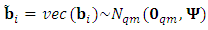, where is unstructured matrix. Moreover, and are assumed to be independent.

Ÿ The marginal distribution of has normal distribution with expectation and dispersion matrix of dimension ;

(2)

The responses can be expressed as where 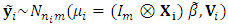, and can be modelled as:

(3)

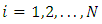
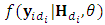
where , and . The p.d.f. of is given by

(4)

It can be verified that

(5)

The complete data likelihood function

Given that the m outcomes are fully observed, the complete-data likelihood function of the parameters, , can be obtained as

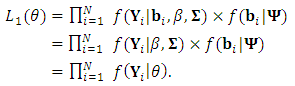(6)

The MLE of can be obtained by maximizing the likelihood function in Eq. (6). Note that this function is based on the marginal distribution function of the response in the absence of the random effects. The random effects can be considered as nuisance parameters as long as the major interest is on the variance structure introduced by . Hence the log-likelihood function, based on Eq. (4) for the whole sample is

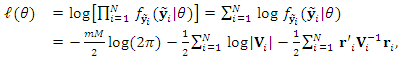(7)

where , is considered the parameter matrix of interest, , while .

A simpler form of the log-likelihood function is given by (Schafer and Yucel, 2002)

(8)

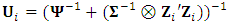
where , and .

We assume that the variance-covariance matrices, and , are unstructured. Moreover, we represent these matrices in terms of their precision form, and . These forms are obtained as linear functions as.

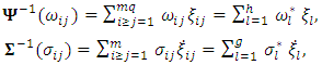(9)

where and is the number of diagnol and off-diagonal elements of . Thus , such that . Similarly, , , and , such that Further, each of and are square matrices of order and m, respectively, with one on the position and zero elsewhere. Hence, the response model parameter vector and the total number of parameters is .

Missing data model and likelihood function

Assume that, for subject i, is subject to non-random dropout at a certain occasion . The responses can be partitioned into two components; the observed part of dimension and missing part of dimension . Also, the response matrix using the operator can be partitioned into two parts; , where , and . Assume that the missing data indicator of dimension where is defined as

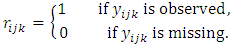For monotone missing data we can define , where 1 is the matrix of ones of dimension and 0 is the matrix of zeros of dimension .

The Diggle and Kenward (1994) model has been proposed for univariate longitudinal data setting. We extend this model to the multivariate longitudinal data of m outcomes. Assume that the dropout of subject i occurs at time denotes the matrix of observed responses history of the m outcomes up to the time , where each of corresponds the row vector of length of observed responses of outcome. Diggle and Kenward (1994) modeled the probability of dropout in terms of the history up to occasion and the possibly missing current response, as This probability is computed for each subject across all occasions as follows:

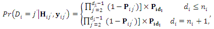(10)

where the logit transformation that is used to model that probability, can be obtained by

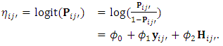(11)

Hence, the dropout probability is obtained via the inverse of the logit transformation as:

(12)

The probability can be computed as

(13)

where is the conditional probability of the missing given the observed responses. Hence the integral in Eq. (13) can be approximated using Monte Carol expectation (Gad and Ahmed, 2006).

The complete-data log-likelihood for the N subjects can be given by

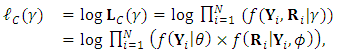(14)

where . Also, it can be re-expressed as

(15)

The MLEs of the parameters can be obtained maximizing each of the two components in Eq. (15) separately. Direct maximization is not feasible because it requires multidimensional integration and maximization (Jason and Xihong, 2002). Numerical and iterative computations are exceedingly required.

3. The Proposed SEM Approach

Maximizion of the log-likelihood function can be carried using iterative approaches to obtain the maximum-likelihood estimates (MLEs) such as Newton-Raphson (NR), Fisher Scoring algorithm(FS), Quasi-Newton (QN) and Expectation-Maximization (EM). Expectation-Maximization algorithm proposed by Dempster et al. (1977). It overcomes the difficulties involved with obtaining MLEs in the presence of missing values. The EM algorithm generally contains of two main steps; an Expectation step (E-step) and a Maximization step (M-step). For more details see McLachlan and Krishnan (2008). The E-step is often difficult to be evaluated. Celuex (1985) proposes the SEM algorithm as an alternative to the EM by replacing the E-step by a simulation step (S-step). Gad and Ahmed (2006) proposed SEM algorithm to fit the univariate longitudinal data in the presence of non-ignorable dropout.

In this article we propose an SEM algorithm to fit the multivariate linear mixed model for multivariate longitudinal data with non-ignorable dropout. The M-step is implemented via two sub-steps. In the first sub-step the Newton-Raphson algorithm is developed to obtain the MLEs of the dropout parameters . In the second sub-step a new type of Quasi-Newton algorithm is proposed to obtain the MLEs of the response parameter .

The S-Step (Simulation step)

Let denotes the missing components of the response matrix over the m outcomes such that indicates the first missing vector, while the second matrix of order is introduced by In this step (the S-step), we simulate m-vector from to represent the responses of the m outcomes at the time of dropout This conditional disribution can be factorized, up to a constant of proportionality, as

(16)

This conditional distribution has no closed form, so direct simulation is not possible. Following the idea of Gad and Ahmed (2006), we suggest using an accept-reject procedure. A vector of length m is simulated from , then it is passed through the following accept-reject procedure;

1. Simulate a candidate m-vector , from the conditional distribution which is m-multivariate normal distribution with parameters and ; the location vector and the dispersion matrix respectively, are given by

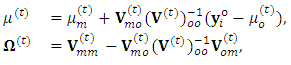(17)

where is the variance matrix corresponds of the observed response matrix ;

2. Compute the m-vector probability of dropout for the candidate vector based on the dropout model

(18)

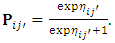
where comprises the m-vector of responses at ; the occasion precedes the dropout occasion. The dropout probability vector, , is evaluated using the inverse transformation in Eq. (12). Then define .

3. Simulate a random m-vector U from uniform distribution over the interval , then take if , otherwise repeat step 1.

We argue that the remaining missing values, following the first missing value, can be considered as missing at random.

The M-Step (Maximization step)

The joint probability function of the pseudo-observed data is

(19)

where . Since does not depend on by construction, the above equation can be simplified to

(20)

Thus the likelihood function for and will be any function of and proportional to . Moreover, based on the selection model, and are assumed to be distinct by definition. Hence, is the same as likelihood .

The M-step of the algorithm comprises two substeps; the logistic step (M1-Step), and the normal step (M2-Step):

The M1-Step (the logistic step):

In this substep the MLEs of the dropout parameter, , is estimated numerically using Newton-Raphson approach. A step halfing algorithm is adopted to guarantee that the log-likelihood function increasing toward the maxima over the iterations. Moreover, in case when the Hessian matrix of is not negative definite, the Newton direction may not point in an ascent direction. Therefore, a modification is adopted using the Levenberg-Marquardt technique, to ensure that the search direction is an ascent direction, hence the algorithm guides the process to the maximum point (Chong and Zak, 2013).

The basic Newton-Raphson algorithm is used to obtain the MLEs for the dropout parameters of the multivariate logistic regression model. The algorithm seeks for optimizing, the log-likelihood function

(21)

where refers to the subjects who complete the study (the completers), hence, refers to dropout subjects. The probabilities vector is computed using Eq. (11) for any occasion , and form Eq. (18) at the occasion of dropout . Implementing the algorithm needs computing the gradient vector and the Hessian matrix . First, the elements of the gradient vector are obtained as follow:

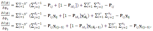where is the m-vector of the responses at occasion j. The elements of the Hessian matrix are obtained as follow:

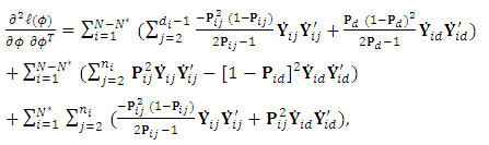where is the response matrix of order .

It is worth noting that at an initial value that might be chosen at which the Hessian matrix is not negative definite, the Levenberg-Marquardt modification of Newton’s algorithm will be adopted. That approach approximates with another matrix , such that , where the scalar is chosen large enough such that is negative definite (Chong and Zak, 2013).

The M2-Step (the normal step):

In this substep the MLEs of the parameters, for the multivariate normal is estimated numerically using a new proposed approach of Quazi-Newton type. The proposed Quazi-Newton algorithm begins with initial values of with , where is computed as

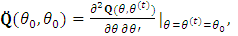(22)

where is the initial values vector of the parameter and the function as in the EM algorithm. Generally, the algorithm proceeds as follows:

1. Initiate the algorithm with , then compute the corresponding and , where is the gradient of the observed log-likelihood function.

2. Compute the step direction vector , then use the line search algorithm to specify that maximizes . The Golden-Section algorithm is adopted here to specify the single parameter that maximize along the search direction d from the point .

3. Set , and compute .

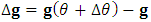4. Based on , and can be evaluated as .

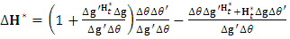5. Replace by , by , and by and return to step (2) or stop based on a stopping criterion.

To implement the above algorithm, the quantities , and are needed. Deviations of such quantities are obtained as follows. First, the EM-quantity, 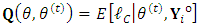, can be easily deduced by taking the expectation of the log-likelihood of the complete-data given the observed responses and the current values of the parameter vector . This function is given by

(23)

where and indicates the complete-data response matrix. To compute this expectation, set 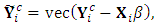where 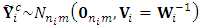. Further the complete-data matrix, , is partitioned into , similarly, 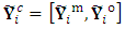. Based on axioms of conditional normal distribution, it can be easily shown that

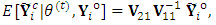where is the square submatrix of corresponding to the observed elements, and is the rectangle sub-matrix of covariances between the missing and the observed elements. On the other hand, it also can be shown that

where is the square submatrix of covariances between the missing elements.

The gradient of the observed log-likelihood, , is derived as

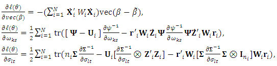where, , and . Further, and are replaced with and , respectively, such that, the scalar which is intensively known as Kronecker delta, equals 1 when and 0 otherwise, where , while .

The second derivatives of the EM-Q function are needed. The computation of the first and the second derivative of the EM-Q function are

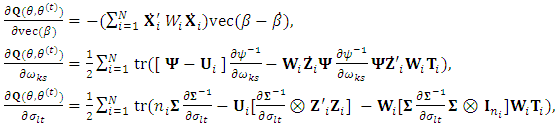where and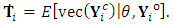

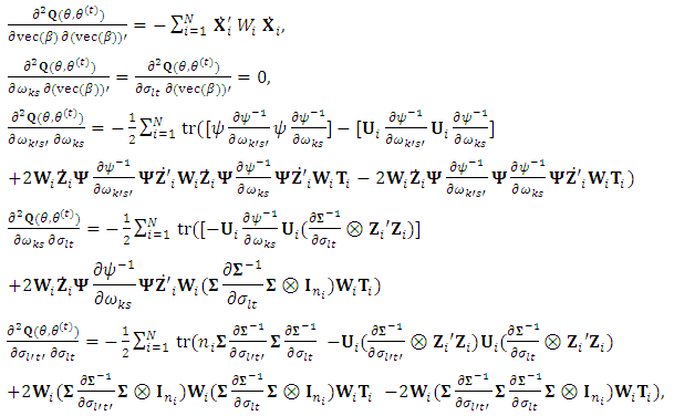For a parameter , the SEM estimates is taken as the mean of the sequence as

(24)

where T is the total number of SEM iterations while is the length of burn-in period.

In the above derivations of the gradient vector and the derivatives of the EM-Q function, the quantities; and are replaced with and , respectively. The scalar is Kronecker delta which equals 1 when and 0 otherwise, where . Similarly the scalar is defined for . The vector is the basis vector of length mq with element equals 1 and all other elements are zeros.

4. Simulation Study

The aim of this simulation is to evaluate the performance of the proposed approach. The evaluation criteria is the relative bias.

Simulation Setting and data generation

Two sample sizes were assumed; , and to generate data. The number of outcomes for each subject is assumed to be three outcomes; . The number of time points is fixed at 10; . The number of replications is chosen as 200. It is assumed that subjects are allocated to one of three treatments A, B, and C. Hence, there are a matrix of dimension of fixed-effects of the three covariates across the three outcomes. The subject-specific design matrix is assumed to have two columns ; the random intercept and slope. Such that, the two subject-specific covariates , for odd subject, and , for even subjects. Also the random design matrix is assumed to be time-invariant. Consequently, the individual level matrix of random-effect parameters is is of order . It represents the parameters of random-effects across outcomes. This matrix is generated for each subject as , where is of dimension assumed to be unstructured matrix. The measurement errors associated with the three outcomes are assumed to be independent over the repeated measure having a common unstructured variance-covariance matrix of dimension . Hence, for each subject the matrix is generated from a matrix normal distribution of parameters 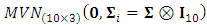. The true value of the elements of the parameter matrices; and are assumed as

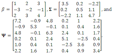The response matrix for each subject, is generated from the model

(25)

The missing data model is

(26)

where each of and is a 3-column vector, indicates the probabilities of dropout at the occasion j associated to the vector of responses, the vector of responses that were planned to be measured at occasion j, and the vector of responses at the previous occasion , respectively. However, if the dropout occasion, for a subject i, is specified as then the dropout probability is computed as a probability of the dropout time at all possible occasion as follow

For each subject, the response matrix generated in the previous step is exposed to a non-random dropping process on the occasion level. Precisely, at occasion j, after the baseline , the response vector has been checked to be whether retained or dropped as follow:

1. The initial values for the parameter vector of logistic dropout model is assumed to be .

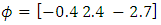2. The probability vector is computed based on Eq. (26).

3. A random variable U is generated from uniform (0,1).

4. The response vector is dropped if , otherwise it is retained.

Simulation Results

The proposed approach introduced has been applied to data. For each of the two maximization steps the stopping criterion that is suggested in Demidenko (2004) is used. Precisely, the iteration will be terminated if the norm value of the absolute difference of two successive values of the gradient vector at fixed parameter values is less that 0.0001. To accelerate the algorithm the study adopted the Levenberg-Marquardt technique to modify each of the Hessian matrix of the dropout parameters and the second derivative matrix of the Q function of the model precision parameters, to be negative definite. The SEM algorithm is iterated for 500 iterations with a burn-in period of 250 iterations. The MLEs for the parameters were taken as the averages of the last 250 iterations. The performance of the proposed approach is evaluated via the relative bias (RB) of its obtained MLEs, which was computed as follow:

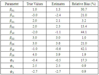
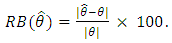The parameter estimates are displayed in Table (1) for N = 25 and Table (2) for N = 50.

Table (1). Parameter estimates for N = 25

Table (2). Parameter estimates for N = 50

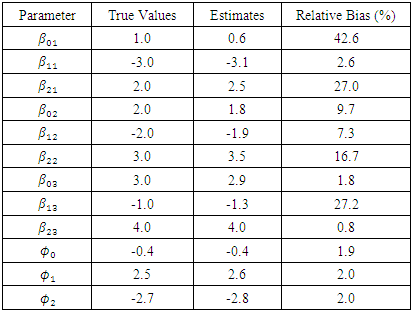
The results show similar performance for the dropout parameter estimates based on the two settings of sample sizes. However, the estimates of the intercept parameter of the first outcome show maximum bias in both tables (30.7%, and 42.6%). For sample size N = 25, the estimate of the effect of the first treatment on the second and third outcomes show somewhat large bias (44.1%, and 42.1% receptively). Generally, the second table show less bias for most parameters (except for the estimate of the first intercept). It almost does not exceed 27.0% approximately. Thus, the proposed approach show higher performance with large sample sizes.

5. Conclusions and Future Research

The study introduces a new estimating approach for modeling multiple outcomes longitudinal data under the multivariate linear mixed model (MLMM) in the presence of non-ignorable missingness. The missing pattern was assumed to be monotone, such that the m outcomes have the same pattern of dropout, while the covariates were assumed to be fully observed. To obtain valid estimates of the model parameters, the study incorporates the model of missing data into the estimation process via the logit selection model. The SEM algorithm is used as estimation approach. The S-Step of the algorithm was implemented via accept-reject principle for simulating the m-vector of outcomes at the dropout occasion from the specified distribution. The algorithm suggested two maximization steps; M1-Step to maximize the likelihood function of the dropout parameters of the multivariate logistic model, and M2-Step to maximize the likelihood function of the response model parameters. The study proposed a novel algorithm to implement the second maximization which is a new form of Quasi-Newton algorithm that incorporates EM-related quantity which is the Q function. The resulted proposed approach is a QN of EM-type.

The proposed approach in efficient in at least major two respects. It suggested using a new version of Quasi-Newton algorithm that embedded with some EM quantities. It takes the advantage of the EM algorithm in handling incomplete data by augmenting the missing and the observed observation to produce better estimates. However, it avoids complicated computation of the EM algorithm due to its iterating on the E-step which is infeasible with models with multi-parameters. So, it suggested computing the matrix of the second derivatives of the Q function with respect to the current guess of the precision parameters only once to initiate the basic Quasi-Newton algorithm.

Some possible extensions to the current study are recommended for further investigation. The current study could be extended assuming the intermittent pattern. Consequently, different likelihood function for the missing data mechanism parameters should be derived to fit such pattern. Moreover, it is very practically to violate the assumption that all outcomes have the same pattern of missingness. Violating such assumption will cause a considerable modification in the computation of the Q function. One further extension is to admit possible missing covariates. This will motivate incorporating missing data mechanism of the covariates into the estimation process.

It is very common to assume that the measurement errors within subjects are autocorrelated. It is possible to extend the variance structure of the errors from to be , where the matrix can take a simple autoregressive pattern. However, this will imply estimating more parameters.

The performance of the proposed approach is evaluated by a simulation study assuming three outcomes. The study is needed to be extended to check its applicability for a higher number of outcomes.