-
Paper Information
- Paper Submission
-
Journal Information
- About This Journal
- Editorial Board
- Current Issue
- Archive
- Author Guidelines
- Contact Us
International Journal of Probability and Statistics
p-ISSN: 2168-4871 e-ISSN: 2168-4863
2018; 7(1): 19-30
doi:10.5923/j.ijps.20180701.03

Heteroscedastic and Homoscedastic GLMM and GLM: Application to Effort Estimation in the Gulf of Mexico Shrimp Fishery, 1984 through 2001
 Abstract
 Reference
 Full-Text PDF
 Full-text HTML
Morteza Marzjarani
NOAA, National Marine Fisheries Service, Southeast Fisheries Science Center, Galveston Laboratory, Galveston, USA
Correspondence to: Morteza Marzjarani , NOAA, National Marine Fisheries Service, Southeast Fisheries Science Center, Galveston Laboratory, Galveston, USA.
| Email: |  |
Copyright © 2018 Scientific & Academic Publishing. All Rights Reserved.
This work is licensed under the Creative Commons Attribution International License (CC BY).
http://creativecommons.org/licenses/by/4.0/

This article presents an overview of the homoscedastic and heteroscedastic Generalized Linear Mixed Model (GLMM) and General Linear Model (GLM). Mathematical relations are defined which map categorical variables onto continuous covariates. It is shown that these relations can be used for different purposes including the addition of pairwise interactions and higher order terms (such as nested terms) to the models. The impacts of these relations on 1984 through 2001 shrimp efforts data in the Gulf of Mexico (GOM), year by year or all years together are compared in the paper. These data sets are also checked for possible heteroscedasticity using Breusch-Pagan and the White’s test. It was observed that these data sets show some degree of the heteroscedasticity. The method of weighted least square (WLS) was applied to these data sets and shrimp efforts were estimated before and after the corrections for the heteroscedasticity were made. In addition, it was shown that both the GLMM and the GLM represent these data sets in a satisfactory manner. Efforts generated via a GLMM and a GLM for both homoscedastic and heteroscedastic models showed that although each data set was heteroscedastic, the severity of the heteroscedasticity was compromised when the data sets 1984 through 2001 were compared.
Keywords: Estimation, General linear models, Generalized linear mixed models, Heteroscedasticity
Cite this paper: Morteza Marzjarani , Heteroscedastic and Homoscedastic GLMM and GLM: Application to Effort Estimation in the Gulf of Mexico Shrimp Fishery, 1984 through 2001, International Journal of Probability and Statistics , Vol. 7 No. 1, 2018, pp. 19-30. doi: 10.5923/j.ijps.20180701.03.
Article Outline
1. Introduction
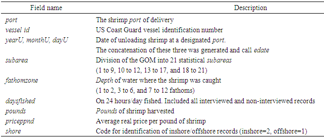
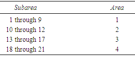
- The purpose of this article was to study the statistical issues related to the effort data files in the northern Gulf of Mexico (GOM). It was not intended to recommend any method for the effort estimation, but rather to examine the 1984 through 2001 shrimp data files for the heteroscedasticity and the possible impact of it on the shrimp effort estimation. The readers are encouraged to read the literature and the current method used to estimate shrimp effort in the GOM by the National Marine Fisheries Service [1].The General Linear Mixed Model (GLMM) is an extension of the General Linear Model (GLM) which in addition to the fixed portion, it also includes a random part. In the GLMM the word “Generalized” indicates that the response variable is not necessarily normal and the word “Mixed” refers to the random effects in addition to the fixed effects in the GLM. The GLMM has been addressed by many authors. Authors in [2] cover a large number of the applications of this model in social sciences. References [3-9] have addressed the generalized linear mixed models extensively. The general linear model has been used to estimate shrimp effort in the Gulf of Mexico (GOM) [10]. Reference [11] extensively applied different aspects of the GLM to estimate the shrimp effort in the GOM for the years 2007 through 2014 including the introduction of a mathematical relation to the model. This article presents an overview of homoscedastic and heteroscedastic models. The GLMM and GLM will be applied to the shrimp data files 1984 through 2001. The mathematical relations presented in [11] are extended and applied to different scenarios including pairwise interactions and nested models. Since the data sets used in the article extend over a period of time (18 years), from a statistical perspective, it is of interest to measure the impact of year on the analysis performed on the data sets. National Marine Fisheries Service (NMFS) is responsible for shrimp effort estimation in the Gulf of Mexico (GOM). NMFS port agents and state trip tickets record the daily operations and shrimp production of the commercial fisheries fleet operating within the boundaries of the U.S. GOM [12]. For assigning fishing activity to a specific geographical location, scientists have subdivided the continental shelf of U.S. Gulf of Mexico into 21 statistical subareas [13]. Subareas 1-9 represent areas off the west coast of Florida, 10-12 represent Alabama/Mississippi, 13-17 represent Louisiana, and 18-21 are designated to Texas (Figure 1). These subareas are further subdivided into 5-fathom depth increments from the shoreline out to 50 fathoms ([1], Page 5). These divisions are used by port agents and the state trip ticket system to assign the location of catches and fishing effort expended by the shrimp fleet on a trip-by-trip basis The shrimp data files include several fields of interest to this study. Table 1 gives the fields used in this research and the corresponding descriptions.
|
2. Methodology
- This study focused only on the offshore records in the shrimp data files 1984 through 2001 in the northern GOM. Since the shrimp data files contained both inshore and offshore data, the first step was to identify and then remove the inshore records from these files. All the records in the shrimp data files 1984 through 2001 with the shore code 2 were removed from these files. Scientists have divided the Gulf of Mexico into 21 statistical subareas as shown (Figure 1).
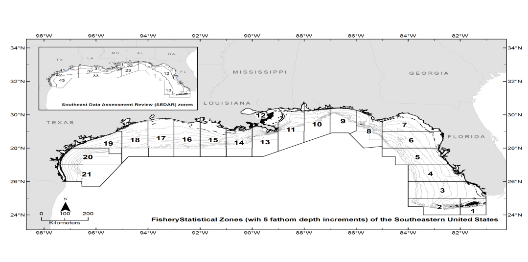 | Figure 1. The Gulf of Mexico is divided into twenty-one statistical areas (1-21) as shown |
 | (1) |
 | (2) |
|
 | (3) |
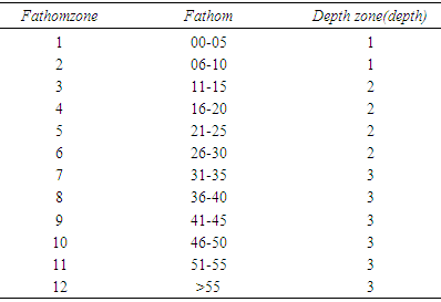
 stands for “Exclusive or Exclusive Disjunction or XOR operator.”As an alternative to using Table 2 to revise fathomzone values above 12, the modes of fathomzone values below 12 for each vessel were found (see formula (4)). Then all fathomzones above 12 per vessel were replaced with the corresponding mode.
  | (4) |
|
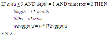 where l<1, p>1, w<1. • To present a more challenging scenario, suppose the experimenter knows from the past that vessels beginning with vessel id number 12345 are considered at least 60 feet long and they usually fish in area 4, at depth 2, and in trimester 1. He/she wishes to set the vessel length at 60 if a length is less than this number. Below is the algorithm for this hypothetical situation.
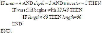 Although, all the examples mentioned above are functions, such relations do not have to be defined as functions and this provides even a greater flexibility to the researcher.In order to develop a GLMM or a GLM for shrimp effort estimation using the 1984 through 2001 data sets individually or collectively, the variables length, lnlbs, wavgppnd, area, depth, and trimester and also the first order interactions between continuous variables were included in the models as described below.
2.1. The Model
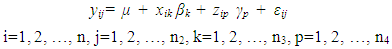
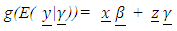
- The model considered in this research is a well-known generalized linear mixed model (GLMM). Algebraically, the model can be written as follows:
 | (5) |
 is the response,
  is the overall mean,
  are constant observations,
  ‘s are error terms, and zip = 1 if i=p; 0 otherwise. It is more convenient to write the equation given in (6) in matrix form.
 | (6) |
 is a column n x1 vector of observations,
 is an n x n1 matrix relating
  is a n1 x 1 column vector of fixed portion of the model. Also,
  is an n x n2 identity matrix relating
  is an n2 x 1 column vector of random portion, and
  is n x 1 column vector of the error terms, the variability in y not explained by the portion
  In (6),
  is the non-random portion of the model,
  is the random effect, and
  is the random error part of the model. As is usually the case, it is assumed that
  is normally distributed with mean 0 and variance covariance
  It is also assumed that
  is normally distributed with mean 0 and variance-covariance
  In this model, the fixed part includes the categorical variables area, depth, trimester, and year (where applicable). The random portion of the model includes the vessel length (length), lnlbs, wavgppnd, and their pairwise interactions or a mathematical relation. The matrices
  and
and  are commonly known as the G-side and the R-side of the model. The random effect determines the G-side of the model variance and it is defined by the RANDOM portion in the model. Furthermore, it is assumed that
  and
and  are uncorrelated. Therefore, one can easily observe that
 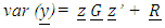 | (7) |
 | (8) |
 , the Identity function is selected for g (.). The reason for having the link function in GLMM is the fact that unlike GLM, the response variable in GLMM does not need to be normally distributed and its range does not have to be in the interval (−∞, +∞). Furthermore, the relationship between predictors and response does not have to be simple relationship. The link function establishes a relationship between these components of the model in such a way that the range of the non-linearly transformed mean g(.) ranges from −∞ to +∞. The model defined in (6) becomes equivalent to a randomized block design if the non-random portion of the model is dropped. Clearly, in the absence of the random portion of the model, equation (6) reduces to a GLM. In the case model (6) contains only the random effects, the
  matrix is of interest. On the other hand, in a model with fixed effects only the
  matrix is of interest. In the absence of the random effects and if
  in the form
  where I is an identity matrix (that is, a homoscedastic model), the GLMM reduces to a GLM or a GLM with overdispersion (this term will be defined later in this article). Using a similar approach as in GLM, that is, maximum likelihood estimation (MLE), the parameters in (6) can be estimated as:
 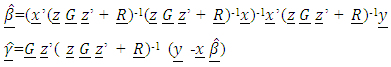 | (9) |
 was considered as follows:
 | (10) |
 are diagonal matrix. In the case of a homoscedastic model,
  is an identity matrix. Some authors have considered some special cases. For example, [14] assumed that the
  matrix for a fixed effect model with two covariates was in the form
  where
where  with
with 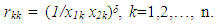 With such choice for the
  matrix, the parameter δ measures the strength of the heteroscedasticity in the model: the lower its magnitude, the smaller the differences between individual variances. Of course, when δ = 0, all the variances are identical (homoscedastic model). In practice, the three values 1/2, 1, and 2 for δ are of particular interest.
 2.2. Investigating the Heteroscedasticity in the Data sets 1984 through 2001
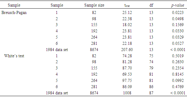
- The word heteroscedastic (sometimes written as heteroskedastic) has a root from the Ancient Greek hetero and skedasis meaning different and dispersion. The term refers to the variability of a variable being unequal across the variable(s) predicting it. It is a major concern in data analysis (such as regression) as it could invalidate the test results among others. It is not surprising to say that to some degree, most (if not all) data sets are heteroscedastic. In most cases like the normality assumptions, researchers take it for granted by assuming that the data sets are homoscedastic. Nevertheless, before fitting a model to a data set and estimating parameters, it seems logical and rather necessary to check for possible heteroscedasticity especially if the sample size is small. To check for possible heteroscedasticity, Breusch, and Pagan, [15], hereafter called Breusch-Pagan, proposed a method known as Lagrange Multiplier (LM). The method was modified by [16] where the normality assumption of the error term was relaxed. The Breusch-Pagan tests the linear form of heteroscedasticity. The White’s test extends this to include non-linear heteroscedasticity and therefore is more general than the Breusch -Pagan test. The issue with the White’s is the addition of new covariates. The test statistic for testing the heteroscedasticity using LM test is:
 | (11) |
 | (12) |
 | (13) |
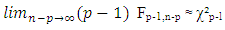 | (14) |
 contained all first order terms of continuous variables and their pairwise interactions and the vector
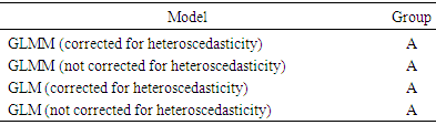
  included all the categorical variables. • For a comparison, a GLM with all first order terms of continuous variables length, lnlbs, wavgppnd and categorical variables area, depth, trimester, and the pairwise interactions of the continuous variables was applied to the Match files.• Both GLMM and GLM were fitted to the 1984 through 2001 and also the combined data files under the assumption of heteroscedasticity and were compared to those under the assumption of homoscedastic models.
 3. Analysis/Results
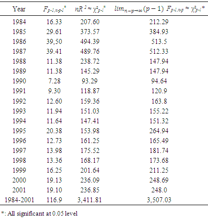
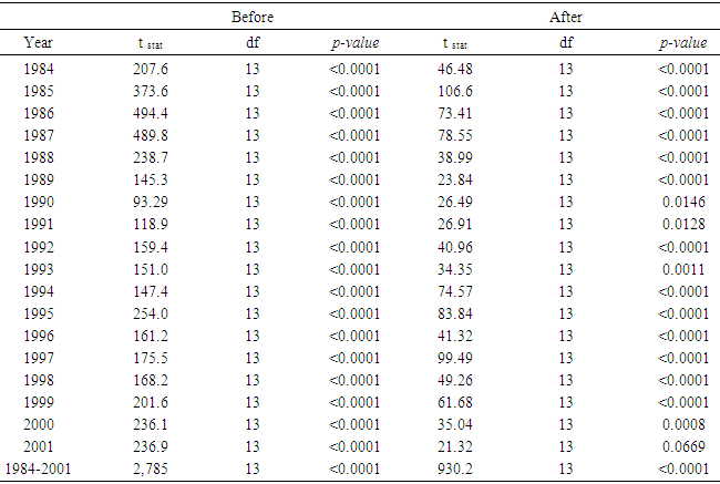
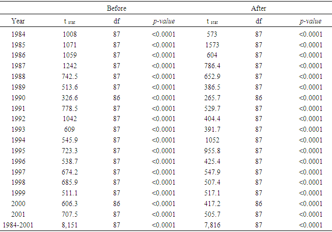
- The objective of this paper was to review the heteroscedastic generalized linear mixed model, and the general linear model, then apply both to 1984 through 2001 shrimp data in the GOM, extend and give some examples of the mathematical relations proposed by [11]. Prior to these, the issue of heteroscedasticity in the shrimp data files 1984 through 2001 was examined. Table 4 displays the results of applying either Formula (11), (12), or (14) to the data sets 1984 through 2001.
|
|
|
|
|
|
|
|
|
|
|
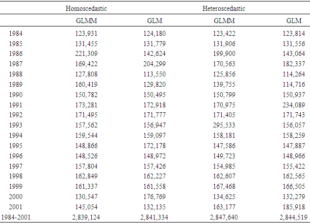
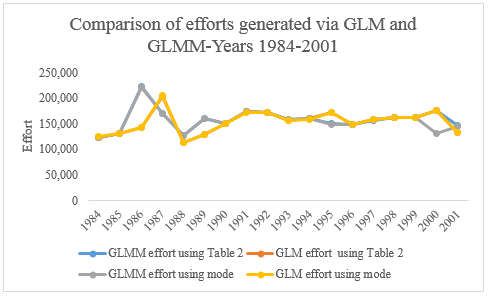 | Figure 2. Efforts generated year by year via a GLMM or a GLM using Table 2 or Formula (4) to revise fathomzones over 12 (under the assumption of homoscedasticity) |
|
|
4. Discussion and Concluding Remarks
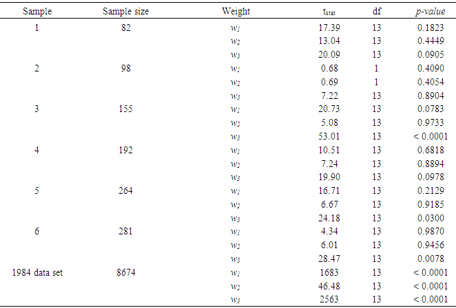
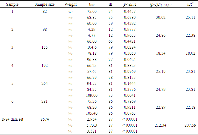
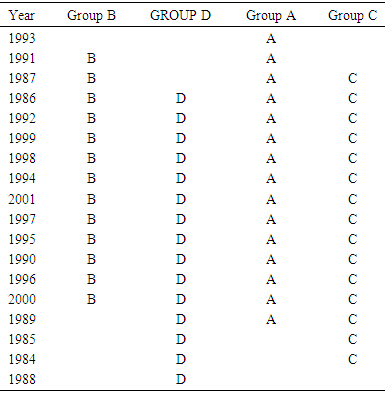
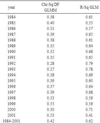
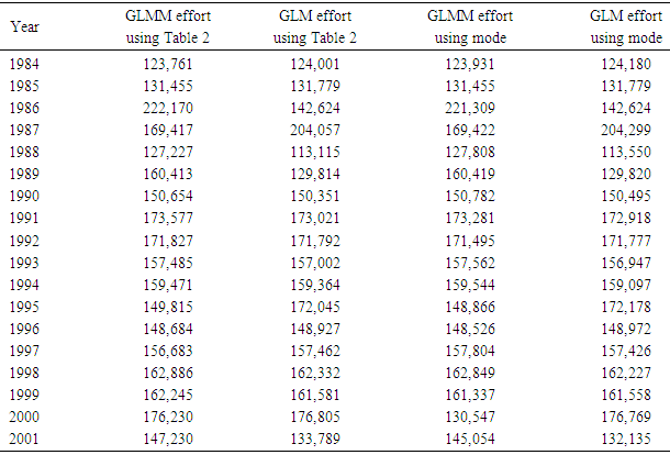
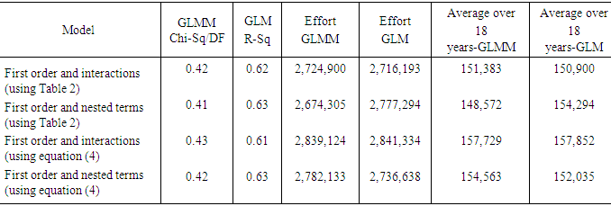
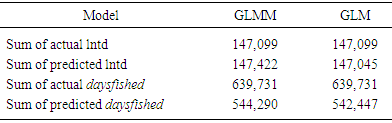
- The goal of this research was to present an overview of the GLMM and the GLM for both homoscedastic and heteroscedastic, to further study the mathematical relations defined in [11] and then to apply these models to the 1984 through 2001 shrimp data files in the GOM. The heteroscedasticity issue is a challenging one to a point that authors usually assumes that the data sets are homoscedastic. Authors in [15] addressed this issue and developed a method for testing the existence of the heteroscedasticity in a data set. Reference [16] modified the method by assuming that the error terms were not necessarily normal also included the non-linear heteroscedasticity in his approach. Clearly, the White’s test is more general, but generates many covariates. The test generally requires higher degrees of freedom and not necessarily consistent with Breusch-Pagan test (Tables 7a and 7b). Reference [17] showed that under certain conditions the two tests are algebraically equivalent. Reference [14] developed an iterative method for estimating the parameters for a heteroscedastic linear regression model with two covariates in a special case. This approach was difficult to deploy here due to a relatively large number of covariates. In this article, the methods proposed by [15, 16] were deployed for testing the existence of the heteroscedasticity in the 1984 through 2001 shrimp data files. It was observed that these data sets include heteroscedasticity. The weighted least square (WLS) method with the inverse of the absolute value of the predicted values from the regression with the residuals as the response (w2) was deployed to correct for the heteroscedasticity. It was concluded that the weight w2 reduced the heteroscedasticity (Tables 7a and 7b). To measure the impact of the heteroscedasticity on the shrimp effort estimation, alternatively efforts were estimated for the years 1984 through 2001 and all years combined under the assumptions of both heteroscedasticity and homoscedasticity. The results showed that over this period, the heteroscedasticity did not cause a significant difference in effort estimation. Clearly, the severity of the heteroscedasticity was compromised by year since the data for each year individually showed the existence of the heteroscedasticity. Under the assumption of homoscedasticity, in the case of the GLMM, the Pearson Chi-Sq/DF ranged from 0.27 to 0.53 where the analysis was performed on the year by year basis. The numerator of this ratio is a quadratic form in the marginal residuals that takes correlations among the data into account. This ratio is known as “overdispersion” which means that the variability in the data is greater than that predicted by the model. Statisticians agree to the definition of this term, but there is no general agreement on the precise interpretation of this quantity (see for example, http://davidakenny.net/cm/fit.htm). Here, I used 1, that is, residual deviance equals its residual degrees of freedom, as the cutoff point to indicate that the variability in the data set has been modeled properly. However, this can easily be challenged. Using this criterion, the GLMM overall represents the data set satisfactorily. Equivalently, GLM produced an R-Sq ranging from 0.41 to 0.79 on the year by year basis. Again, this could be interpreted as a satisfactory model. Efforts for both GLMM and GLM were estimated using nested models with year as a variable. A word of caution is in place here. Both models are very computer extensive and require a relatively high computing power due to a large number of parameters in the models and also the volume of the data set generated when the data for the years 1984 through 2001 are combined (the number of significant parameters in GLMM and GLM were 78 and 108 respectively). Further review of the estimates given in Table 11 showed that there was no significant difference between efforts generated using Table 2 or equation (4). That is, revising the fathomzones above 12 using either Table 2 or equation (4) produce the same or equivalent results. A few possibilities for the models as well as the mathematical relations were considered in this paper. Examples for the relations were not intended to generate efforts, but to show how these relations can be used in case, for example, the experimenter wishes to modify the model by adding arbitrary terms to it or to handle other issues such as the outliers in the data file.The heteroscedasticity issue is a challenging one and most data analysts do not check the data sets in that respect. Like to normality assumptions, it is usually taken for granted and data sets are assumed homoscedastic. However, most data sets are heteroscedastic to some degree and need to be checked and proper adjustments (if needed) be made before any analysis is performed. The issue becomes more challenging when dealing with large data sets as the test statistics tend to increase along with the sample size. Once the heteroscedasticity was detected, the next step is to develop a proper weight function to correct the heteroscedasticity, which in turn presents a challenge. It was concluded that a GLMM with first order of categorical variables as the fixed effect portion and first order and pairwise interactions of continuous variables or a GLM with the same categorical and continuous terms present this data file adequately with a slight edge given to the GLM (based on my interpretation of the dispersion parameter). However, one must always be cautious not to claim that the proposed models are “perfect.” A quote from a well-known statistician [18] seems appropriate here. “Essentially, all models are wrong, but some are useful.” Although, the application was limited to the shrimp data in this article, it could be easily applied to other data sets. Heteroscedasticity is common among most data sets and this paper should be helpful in other areas of research.(1) References to any software packages throughout this article do not imply the endorsement of the said products.
Disclaimer
- The scientific results and conclusions, as well as any views or opinions expressed herein, are those of the author and do not necessarily reflect those of NOAA or the Department of Commerce.