-
Paper Information
- Previous Paper
- Paper Submission
-
Journal Information
- About This Journal
- Editorial Board
- Current Issue
- Archive
- Author Guidelines
- Contact Us
International Journal of Probability and Statistics
p-ISSN: 2168-4871 e-ISSN: 2168-4863
2018; 7(1): 14-18
doi:10.5923/j.ijps.20180701.02

Detection of Outliers in Growth Curve Models: Using Robust Estimators
 Abstract
 Reference
 Full-Text PDF
 Full-text HTML
O. Ufuk Ekiz
Department of Statistics, Gazi University, Ankara, Turkey
Correspondence to: O. Ufuk Ekiz, Department of Statistics, Gazi University, Ankara, Turkey.
| Email: |  |
Copyright © 2018 Scientific & Academic Publishing. All Rights Reserved.
This work is licensed under the Creative Commons Attribution International License (CC BY).
http://creativecommons.org/licenses/by/4.0/

Outliers cause problems in statistical inferences for statistical analysis as well as growth curve model (GCM)s. Hence, robust estimators could be used to construct more significant inferences and this would make it possible to detect outliers more accurately. In this study, the method of least median square (LMS) is adopted to GCM. Then LMS, M, and ML (maximum likelihood) estimators are applied to real data applications and the reasons for the differences in the results are discussed.
Keywords: Growth curve model, Outlier, Robust
Cite this paper: O. Ufuk Ekiz, Detection of Outliers in Growth Curve Models: Using Robust Estimators, International Journal of Probability and Statistics , Vol. 7 No. 1, 2018, pp. 14-18. doi: 10.5923/j.ijps.20180701.02.
Article Outline
1. Introduction
- Growth curve model (GCM) is a generalized multivariate variance model and is defined by Potthof and Roy [1] so as to model longidutional data. This model is studied by several authors in literature as well [2-4]. Applications of this model to especially economic, social, and medicine sciences would give opportunities to investigate the mean growth in a population over a short period of time. Hence, making short term predictions become feasible by employing this model.Let X and Z be the well-known design matrixes with ranks m<p and r<n, respectively. p is the number of time points observed on each of n cases. GCM is given by
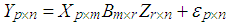 | (1) |
 is the observation matrix and B is the parameter matrix. Moreover,
  denotes the error matrix where the columns are p-variate normally distributed independent variables with mean 0 and unknown covariance matrix
  , [5]. Hence,
 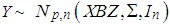 and I is the identity matrix. However, existing outliers in the data would impact on statistical inferences as they do in statistical analysis. Outlier is an observation that deviates from the rest of the data [6]. To get rid of the negative impacts of these outlying points there are two commonly addressed approaches. First group of methods are the so-called statistical diagnostics [7, 8]. The main purpose of these methods is based on observing the variation that an observation (or a group of observations) do have on the measure so as to point out as effective. However, for the sake of reliability of these approaches masking and swamping problems should not be ignored. The methods, through which the outliers are detected by means of robust estimators conduct the second group approaches [9]. In recent years, these are particularly preferred in statistical analysis. Since they are not likely to account the outliers (or attain minimum weights to them) in calculations of robust estimators, measures used for detection of outliers would not (or minimum) be affected.Even though studies on the determination of points outlying of the bulk began long ago, it is only after 1990 that it has started to improve [10-14]. The purpose of this paper is to identify outliers in GCMs by using robust estimators least median squares (LMS) and M. Section 2 emphasis on the M estimator and the adaptation of LMS to GCM as well. In Section 3, we explained how to determine outliers by means of residuals. Finally, two real-life applications including outliers are considered to confirm differences on identifying them by means of residuals based on robust and non-robust estimators.
2. Parameter Estimations in Growth Curve Model
- The ordinary least square (OLS) estimator of parameter B in equation (1) is
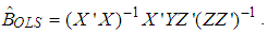 | (2) |
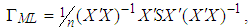
 , the estimator of parameter
  which is denoted as
  , [5], is calculated from
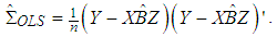 | (3) |
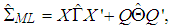
 is of Rao’s simple covariance structure (SCR), i.e.,
 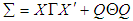 , where both
  and
and 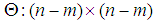 are unknown positive definite matrices, and
  .
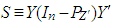
.  is the orthogonal matrix space of X defined by
 | (4) |
 and
and  are
are 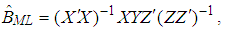 | (5) |
 | (6) |
 | (7) |
 | (8) |
 and
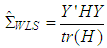
and 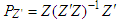 , [12, 16].Let us now describe the weighted least square (WLS) estimator
 | (9) |
 . Here,
  denotes the residual of the ith observation and
  | (10) |
 | (11) |
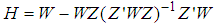 [17]. W is a diagonal matrix that consists of weights attained for each observation and “tr” denotes the trace of the corresponding matrix. Define
 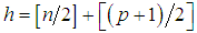 and t as a value that ranges from 1 to
  .
.  denotes the number of h-combinations from a given set of n elements. The LMS estimators
  and
and  are obtained from equations (9) and (11), respectively, by minimizing the objective function
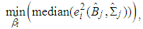 | (12) |
 and
and  , [9]. Moreover, the weight matrix
  , which will be used for the underlined equations, is determined so that its ith diagonal element
  is
is 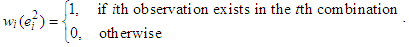 When
When  . is used as the initial point and the value
  is obtained from the kth iteration of
  ,
,  will be the M estimator,
  .
.  function has a minimum at “0” for all values of
  . Here, Tukey’s
  function (bi-square), [18, 19], is used to compute the M estimator. Hence, the ith diagonal element
  of the weight function
  that should be used both in equation (9) and (11) would be
 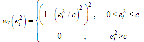 | (13) |
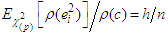 , where
  is the expected value obtained from chi-squared distribution with p degrees of freedom. Here,
  value is preferred so as to have the same breakdown point as the LMS estimator.
3. Detecting Outliers in Growth Curve Model
- It is known that the sum of squared residuals fit to chi-square with p degrees of freedom when the data does not contain outliers [20]. Hence,
 | (14) |
 | (15) |
 the ith observation would be identified as an outlier.
  denotes the significance level.
  and
and  are the estimators of parameters
  and
and  , respectively, and are calculated from an any estimation method. However, if estimators are affected by outliers they would cause for determining wrong observations as outliers. Therefore, robust estimators that are less likely to be affected by outlying points should be preferred and this would assure more reliable results.
4. Example Applications
- Understanding the importance of selection of estimators in parameter estimates and detection of outliers in GCMs, two real data sets are examined.
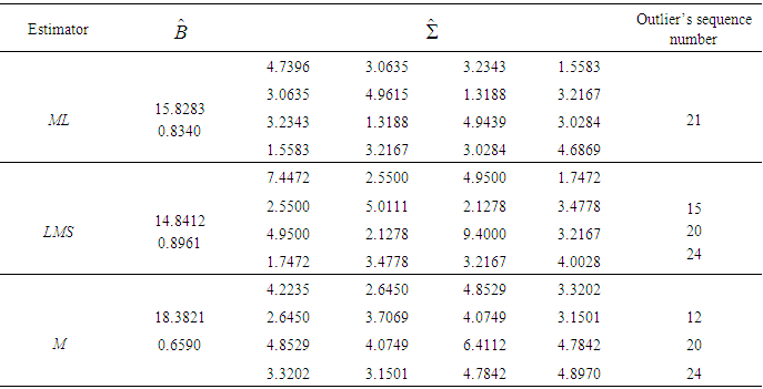
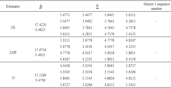
4.1. Dental Data
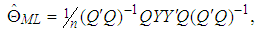
- This data set, was first considered by Potthoff and Roy, [1], and later analyzed by several authors (see [21-24]). Dental measurements were made on 11 girls and 16 boys at ages 8, 10, 12, and 14 years. Each measurement is the distance in millimetres from the centre of the pituitary to the pterygomaxillary fissure. Sequence number to each measurement is assigned. Then, the ML, LMS, and M estimators of this data set are computed for boys and girls separately, and are given in Table 1 and Table 2. The sequence numbers of detected outliers are summarized in the last column of these tables as well. As it shown in Table 1 by means of ML estimator, observation numbered 21 is an outlier. On the other hand, outliers based on LMS and M estimators are observations numbered as 12, 15, 20, and 24. ML estimators are non-robust, so they are greatly affected by outliers in data. Furthermore, by examining the girl’s data there are no outliers (see Table 2).
|
|
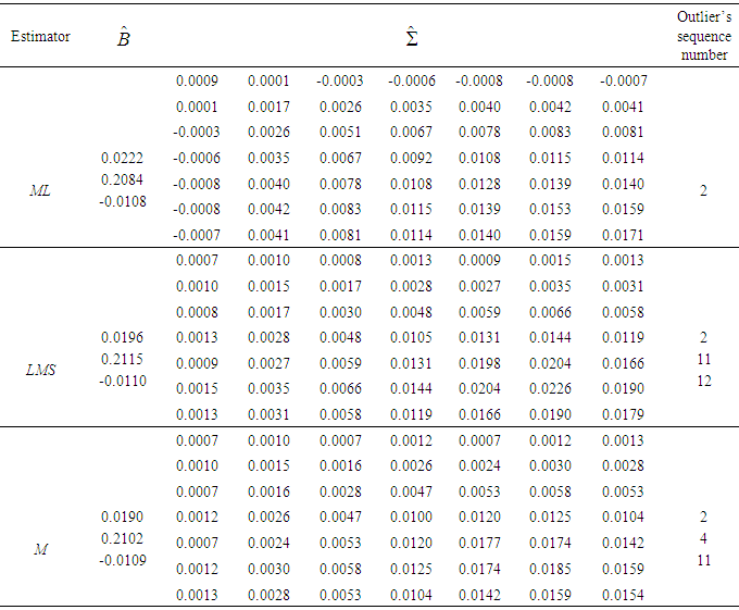
4.2. Mouse Data
- This data set is reported by Izenman and Williams, [25], and is analyzed by Roo and Lee as well [22-24]. It consists of weights of 13 male mice measured at intervals of 3 days over the 21 days from birth to weaning. As done to the dental data, sequence number to each measurement is assigned. The ML, LMS, and M estimators of parameters B and
 for this data set are given in Table 3. The sequence numbers of the detected outliers obtained by using these estimators are also determined. From the table, it is noticeable that robust estimators’ performance on detecting outliers differs from ML estimators. ML estimators have detected only the second observation as an outlier while robust estimators have detected 4th, 11th, and 12th observations as outliers.
|
5. Conclusions
- ML estimators in GCMs both using for comparison of groups and making short term predictions could be badly affected by outliers in data. This affection can lead to bad estimates of parameters for the assumed distribution of the data. Moreover, utilizing non-robust ML in hypothesis tests to determination of outliers will give misleading results as well. When the investigation of outliers is based on robust test statistics, it is well-known that the obtained results could reflect the reality much better. In Section 4, two data sets that are used in literature for different purposes are analyzed. Accordingly, the results differ to a great extend when using robust or non-robust estimators. Moreover, the variance of robust M estimator is smaller than LMS’s. Hence, obtaining results with robust M estimator will be more convenient.