Rama Shanker
Department of Statistics, Eritrea Institute of Technology, Asmara, Eritrea
Correspondence to: Rama Shanker, Department of Statistics, Eritrea Institute of Technology, Asmara, Eritrea.
| Email: |  |
Copyright © 2017 Scientific & Academic Publishing. All Rights Reserved.
This work is licensed under the Creative Commons Attribution International License (CC BY).
http://creativecommons.org/licenses/by/4.0/

Abstract
In this paper, a one parameter lifetime distribution named “Suja distribution” for modeling lifetime data, has been proposed and investigated. Important properties of the proposed distribution including its shape, moments, skewness, kurtosis, hazard rate function, mean residual life function, stochastic ordering, mean deviations, Bonferroni and Lorenz curves, and stress-strength reliability have been discussed. The condition under which Suja distribution is over-dispersed, equi-dispersed and under-dispersed have been studied and compared with other one parameter lifetime distributions. The estimation of the parameter has been discussed using maximum likelihood estimation and method of moments. Finally the goodness of fit of the proposed distribution has been discussed with a real lifetime data and the fit has been compared with other one parameter lifetime distributions.
Keywords:
Lifetime distribution, Moments, Hazard rate function, Mean residual life function, Mean deviations, Stochastic ordering, Bonferroni and Lorenz curves, Stress-strength reliability, Estimation of parameter, Goodness of fit
Cite this paper: Rama Shanker, Suja Distribution and Its Application, International Journal of Probability and Statistics , Vol. 6 No. 2, 2017, pp. 11-19. doi: 10.5923/j.ijps.20170602.01.
1. Introduction
The modeling and analyzing lifetime data are essential in many applied sciences including medicine, engineering, insurance and finance, amongst others. The two important one parameter lifetime distributions namely exponential and Lindley (1958) are popular for modeling lifetime data from biomedical science and engineering. But, Shanker et al (2015) have conducted a comparative study on modeling of lifetime data from various fields of knowledge and observed that there are many lifetime data where these two distributions are not suitable due to their shapes, nature of hazard rate functions, and mean residual life, amongst others. Recently, Shanker (2015 a, 2015 b, 2016 a, 2016 b, 2016 c, 2016 d) has introduced some one parameter lifetime distributions namely, Akash, Shanker, Amarendra, Aradhana, Sujatha, and Devya, and showed that these distributions give better fit than the classical exponential and Lindley distributions. Each of these lifetime distributions has advantages and disadvantages over one another due to its shape, hazard rate function and mean residual life function. There are many situations where these distributions are not suitable for modeling lifetime data from theoretical or applied point of view. Therefore, an attempt has been made in this paper to obtain a new distribution which is flexible than these one parameter lifetime distributions including Akash, Shanker, Amarendra, Aradhana, Sujatha, Devya, Lindley and exponential for modeling lifetime data in reliability and in terms of its hazard rate shapes. The new one parameter lifetime distribution is based on a two- component mixture of an exponential distribution having scale parameter  and a gamma distribution having shape parameter 5 and scale parameter
  with their mixing proportion
  . The probability density function (p.d.f.) of a new one parameter lifetime distribution can be introduced as
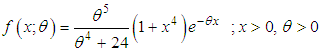 | (1.1) |
We would call this distribution, “Suja distribution”. This distribution can be easily expressed as a mixture of exponential  and gamma
  with mixing proportion
 . We have
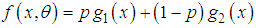 where
where 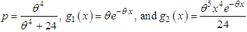 .The corresponding cumulative distribution function (c.d.f.) of (1.1) can easily be obtained as
  | (1.2) |
The graph of the p.d.f. and the c.d.f. of Suja distribution for varying values of the parameter  are shown in figures 1 and 2.
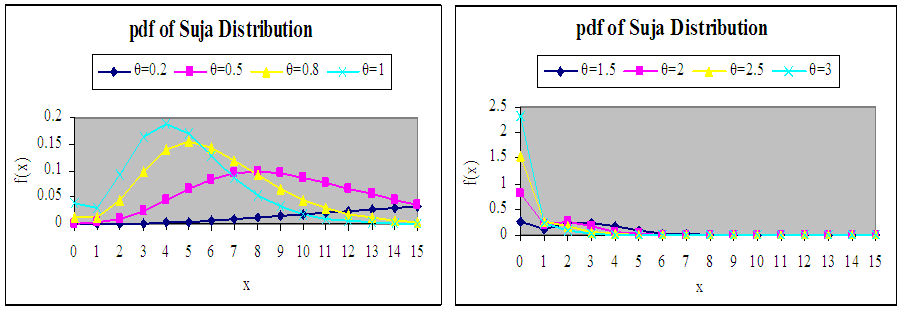 | Figure 1. Graph of the pdf of Suja distribution for varying values of the parameter θ |
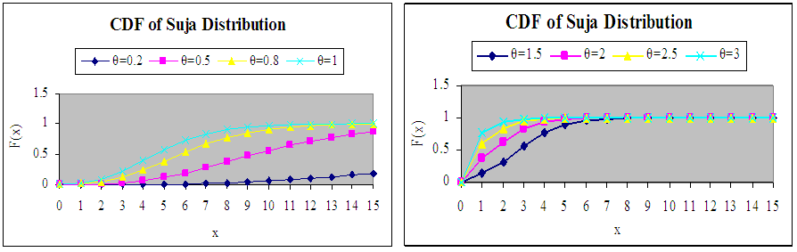 | Figure 2. Graph of the cdf of Suja distribution for varying values of the parameter θ |
2. Moments and Associated Measures
The moment generating function of Suja distribution (1.1) can be obtained as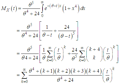 Thus the rth moment about origin of Suja distribution can be given by
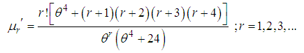 | (2.1) |
Substituting 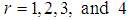 in (2.1), the first four moments about origin of Suja distribution are obtained as
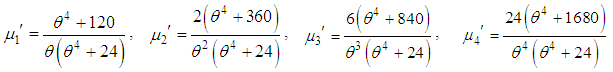 Now using relationship between central moments and moments about origin, the central moments of Suja distribution are obtained as
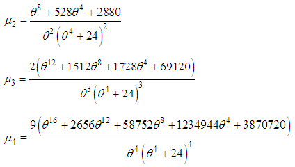 The coefficient of variation
  , coefficient of skewness
  , coefficient of kurtosis
  and index of dispersion
  of Suja distribution are thus obtained as
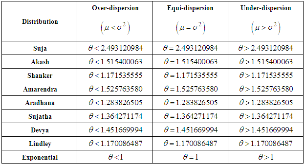
 The condition under which Suja distribution is over-dispersed, equi-dispersed, and under-dispersed has been discussed along with condition under which Akash, Shanker, Amarendra, Aradhana, Sujatha, Devya, Lindley and exponential distributions are over-dispersed, equi-dispersed, and under-dispersed and are presented in table 1.
Table 1. Over-dispersion, equi-dispersion and under-dispersion of Suja, Akash, Shanker, Amarendra, Aradhana, Sujatha, Devya, Lindley and exponential distributions for parameter θ
 |
| |
|
3. Hazard Rate Function and Mean Residual Life Function
Let  and
and  be the p.d.f. and c.d.f of a continuous random variable
  . The hazard rate function (also known as the failure rate function) and the mean residual life function of a continuous random variable
  are respectively defined as
 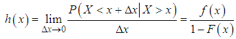 | (3.1) |
and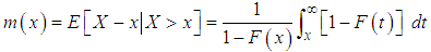 | (3.2) |
The corresponding hazard rate function,  and the mean residual life function,
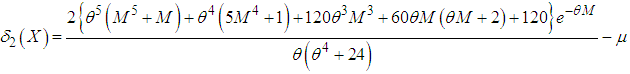
  of the Suja distribution are obtained as
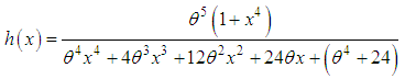 | (3.3) |
and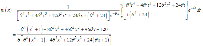 | (3.4) |
It can be easily verified that 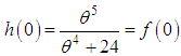 and
and  . It is also obvious from the graphs of
  and
and  that
that  is an increasing and decreasing function of
  , and
, and  , whereas
  is always decreasing function of
  , and
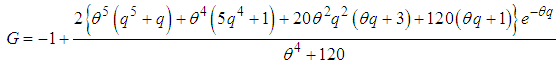
, and  . The graph of the hazard rate function and mean residual life function of Suja distribution are shown in figures 3 and 4.
 | Figure 3. Graph of hazard rate function of Suja distribution for varying values of the parameter θ |
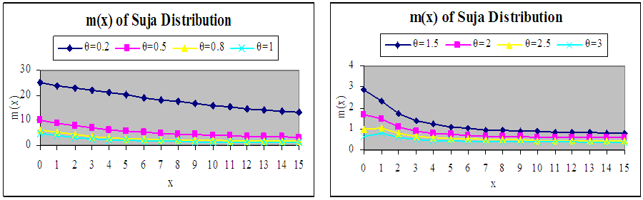 | Figure 4. Graph of mean residual life function of Suja distribution for varying values of the parameter θ |
4. Stochastic Orderings
Stochastic ordering of positive continuous random variable is an important tool for judging their comparative behavior. A random variable  is said to be smaller than a random variable
  in the (i) stochastic order
  if
if  for all
  (ii) hazard rate order
  if
if  for all
  (iii) mean residual life order
  if
if  for all
  (iv) likelihood ratio order
  if
if  decreases in
  .The following results due to Shaked and Shanthikumar (1994) are well known for establishing stochastic ordering of distributions
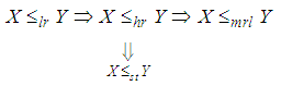 | (4.1) |
The Suja distribution is ordered with respect to the strongest ‘likelihood ratio’ ordering as shown in the following theorem:Theorem: Let  Suja distribution
 and
and  Suja distribution
  . If
. If  , then
  and hence
 ,
,  and
and  .Proof: We have
 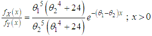 Now
Now 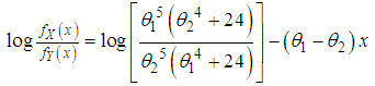 This gives
 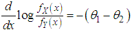 .Thus for
  ,
,  . This means that
  and hence
  ,
,  and
and .
.
5. Mean Deviations
The amount of scatter in a population is measured to some extent by the totality of deviations usually from mean and median. These are known as the mean deviation about the mean and the mean deviation about the median defined as and
and  , respectively, where
  and
and  . The measures
  and
and  can be calculated using the simplified relationships
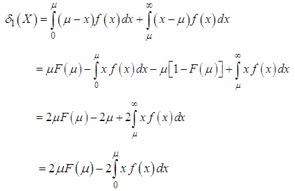 | (5.1) |
and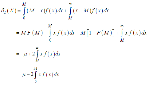 | (5.2) |
Using p.d.f. (1.1) and expression for the mean of Suja distribution (1.1), we get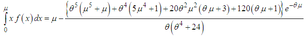 | (5.3) |
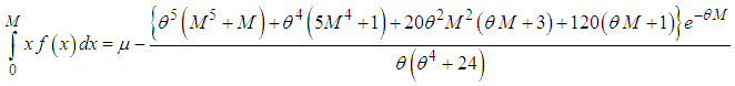 | (5.4) |
Using expressions from (5.1), (5.2), (5.3), and (5.4), the mean deviation about mean,  and the mean deviation about median,
  of Suja distribution (1.1) are obtained as
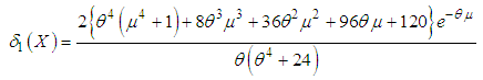 | (5.5) |
 | (5.6) |
6. Bonferroni and Lorenz Curves
The Bonferroni and Lorenz curves (Bonferroni, 1930) and Bonferroni and Gini indices have applications not only in economics to study income and poverty, but also in other fields like reliability, demography, insurance and medicine. The Bonferroni and Lorenz curves are defined as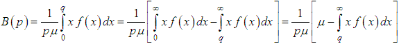 | (6.1) |
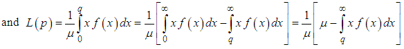 | (6.2) |
respectively or equivalently  | (6.3) |
 | (6.4) |
respectively, where  and
and  .The Bonferroni and Gini indices are thus defined as
 | (6.5) |
 | (6.6) |
respectively.Using p.d.f. of Suja distribution (1.1), we have 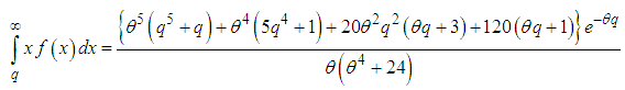 | (6.7) |
Now using equation (6.7) in (6.1) and (6.2), we have 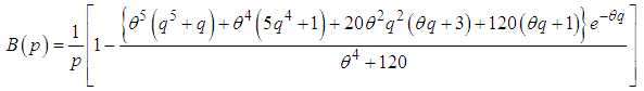 | (6.8) |
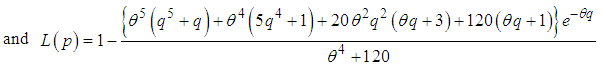 | (6.9) |
Now using equations (6.8) and (6.9) in (6.5) and (6.6), the Bonferroni and Gini indices are obtained as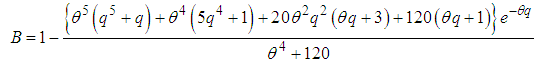 | (6.10) |
 | (6.11) |
7. Stress-Strength Reliability
The stress- strength reliability gives the idea about the life of a component which has random strength  that is subjected to a random stress
  . When the stress applied to it exceeds the strength, the component fails instantly and the component will function satisfactorily till
  . Therefore,
 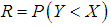 is a measure of the component reliability and in statistical literature it is known as stress-strength parameter. It has wide applications in almost all areas of knowledge especially in engineering such as structures, deterioration of rocket motors, static fatigue of ceramic components, aging of concrete pressure vessels etc.Let
  and
and  be independent strength and stress random variables having Suja distribution (1.1) with parameter
  and
and  respectively. Then the stress-strength reliability
  of Suja distribution can be obtained as
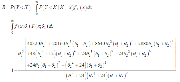
8. Estimation of Parameter
8.1. Maximum Likelihood Estimate (MLE)
Let  be a random sample from Suja distribution (1.1). The likelihood function,
  of (1.1) is given by
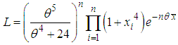 The natural log likelihood function is thus obtained as
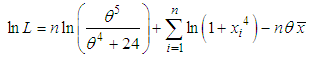 Now
Now 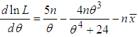 , where
  is the sample mean.The MLE
  of
of  is the solution of the equation
  and so it can be obtained by solving the following fifth degree polynomial equation
 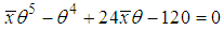 | (8.1.1) |
8.2. Method of moment Estimate (MOME)
Equating the population mean of the Suja distribution (1.1) to the corresponding sample mean, MOME , of
, of  is the same as given by equation (8.1.1).
9. Goodness of Fit
In this section, the goodness of fit of Suja distribution has been discussed with a real lifetime data set from engineering and the fit has been compared with one parameter lifetime distributions namely Akash, Shanker, Amarendra, Aradhana, Sujatha, Devya, Lindley and exponential.The data set is the strength data of glass of the aircraft window reported by Fuller et al (1994) and are given as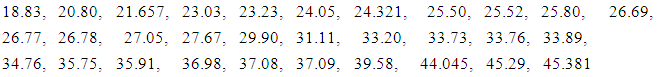 In order to compare lifetime distributions,
  , AIC (Akaike Information Criterion) and K-S Statistics (Kolmogorov-Smirnov Statistics) for the above data set have been computed. The formulae for computing AIC and K-S Statistics are as follows:
 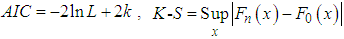 , where k = the number of parameters, n = the sample size and
  is the empirical distribution function. The best distribution is the distribution which corresponds to lower values of
  , AIC, and K-S statistics. The MLE
  with the standard error, S.E
 of
of  ,
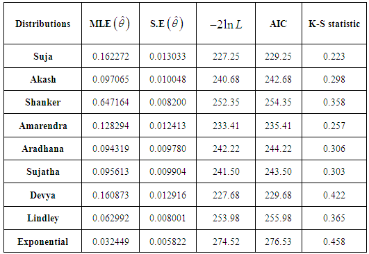
,  , AIC and K-S Statistic of the fitted distributions are presented in the table 2.
Table 2. MLE’s, S.E
 - 2ln L, AIC and K-S Statistics of the fitted distributions of the given data set - 2ln L, AIC and K-S Statistics of the fitted distributions of the given data set
 |
| |
|
It can be easily observed from above table that Suja distribution gives better fit than the fit given by Akash, Shanker, Amarendra, Aradhana, Sujatha, Devya, Lindley and exponential distributions and hence it can be considered as an important lifetime distribution for modeling lifetime data.
10. Concluding Remarks
A one parameter lifetime distribution named, “Suja distribution” has been proposed. Its statistical properties including shape, moments, skewness, kurtosis, hazard rate function, mean residual life function, stochastic ordering, mean deviations, Bonferroni and Lorenz curves and stress-strength reliability have been discussed. The condition under which Suja distribution is over-dispersed, equi-dispersed, and under-dispersed are presented along other one parameter lifetime distributions. Maximum likelihood estimation and method of moments have been discussed for estimating its parameter. Finally, the goodness of fit test using K-S Statistics (Kolmogorov-Smirnov Statistics) for a real lifetime data has been presented and the fit has been compared with some one parameter lifetime distributions and the fit given by the proposed distribution is quite satisfactory.
ACKNOWLEDGEMENTS
The author is grateful to the editor- in - chief and the anonymous reviewer for constructive comments which improved the quality and presentation of the paper.
Note
The paper is named “Suja distribution” by taking the first two letters of my lovely mother Sushila Devi and the first two letters of my great father Janardan Sharma.
References
| [1] | Bonferroni, C.E. (1930): Elementi di Statistca generale, Seeber, Firenze. |
| [2] | Fuller, E.J., Frieman, S., Quinn, J., Quinn, G., and Carter, W. (1994): Fracture mechanics approach to the design of glass aircraft windows: A case study, SPIE Proc 2286, 419-430. |
| [3] | Lindley, D.V. (1958): Fiducial distributions and Bayes’ theorem, Journal of the Royal Statistical Society, Series B, 20, 102- 107. |
| [4] | Shaked, M. and Shanthikumar, J.G. (1994): Stochastic Orders and Their Applications, Academic Press, New York. |
| [5] | Shanker, R., Hagos, F, and Sujatha, S. (2015): On modeling of Lifetimes data using exponential and Lindley distributions, Biometrics & Biostatistics International Journal, 2 (5), 1-9. |
| [6] | Shanker, R. (2015 a): Akash distribution and its Applications, International Journal of Probability and Statistics, 4(3), 65 – 75. |
| [7] | Shanker, R. (2015 b): Shanker distribution and its Applications, International Journal of Statistics and Applications, 5(6), 338 – 348. |
| [8] | Shanker, R. (2016 a): Amarendra distribution and its Applications, American Journal of Mathematics and Statistics, 6(1), 44 – 56. |
| [9] | Shanker, R. (2016 b): Aradhana distribution and its Applications, International Journal of Statistics and Applications, 6(1), 23 – 34. |
| [10] | Shanker, R. (2016 c): Sujatha distribution and its Applications, Statistics in Transition-new series, 17(3), 1 – 20. |
| [11] | Shanker, R. (2016 d): Devya distribution and its Applications, International Journal of Statistics and Applications, 6(4), 189 – 202. |

 Abstract
 Reference
 Full-Text PDF
 Full-text HTML