1. Introduction

Longitudinal studies are not uncommon in biomedical research and social sciences. In such studies each individual (experimental unit) is measured repeatedly over time for the same response variable (outcome) either under different conditions, or at different times, or both. Longitudinal studies are subject to missing values. The missing values are termed dropout if the subject withdraws from the study at certain time without any observed value for it after that specified time. This is called monotone pattern for missing data. If the subject withdraws occasionally, then we have intermittent missing process and a non-monotone pattern.

In the presence of missing data, the validity of any estimation method requires certain assumptions about the reasons behind the missingness; which are the missing data mechanism. Incorporating the missing data mechanism in statistical model means including an indicator variable, R, that takes the value 1 if an item is missing and 0 otherwise. Following Rubin's taxonomy [1], the missing data mechanism is said to be missing not at random (MNAR) if R depends on missing data and may depend on the observed data. In likelihood context this mechanism is labeled as non-ignorable.

The likelihood estimation, especially in the presence of missing values, is intractable as integration over the random effects is required. Moreover, assuming non-normal distribution for the random effects makes the likelihood more complex and it cannot be expressed in closed form. Various approximation methods to evaluate the likelihood integrations were introduced. These include analytical approximation such as the penalized quasi-likelihood (PQL) and numerical integration such as Gauss-Hermite quadrature. Also a lot of iterative simulation techniques based on the EM algorithm have been used to optimize the likelihood function. The Monte Carlo EM algorithm was introduced to estimate likelihood parameters specially when sampling from conditional distribution of random effects or missing data is difficult.

Violation of the normality assumption of random effects has been studied in literature. [2] uses a mixture of normals for the random effects density. [3] and [4] assume that the random effects distribution has a smooth but unspecified density, that can be estimated using semi-nonparametric representation. [5] replaces the normal distribution in linear mixed models by a skew-t distribution. [6] propose replacing the normal distribution with a mixture of normal distributions where the weights of the mixture components are estimated using a penalized approach. They also use the log-normal and gamma distribution for the random effects density. [7] estimate the maximum likelihood parameters for the logistic model when random effects follow a log normal distribution using a Monte Carlo EM (MCEM) algorithm.

Many studies have been emerged focusing on estimating the GLMM parameters in the presence of missing data. [8] use a shared parameter model where an individual's random slope has been used as a covariate in a probit model for the censoring process. [9] propose conditioning on the time to censoring, and use censoring time as a covariate in random effects model. [10] approximate the generalized linear model using a generalized linear mixed model by conditioning the response variable on the missingness data. [11] develop a Monte Carlo EM algorithm to estimate parameters of GLMM with non-ignorable missing response data, with a normal random effects model. [12] propose a latent class model, which is an alternative approach to a pattern mixture model, by assuming that the dropout time belongs to unobserved (latent) class membership. [13] develop the stochastic EM-algorithm (SEM) algorithm for parameter estimation of a GLM in the presence of intermittent non-random missing values. [14] propose a pseudo likelihood method to estimate parameters for longitudinal data with binary outcome and categorical covariates. They assume missing not at random mechanism and non-monotone pattern. [15] propose a class of unbiased estimating equations using the pairwise conditional technique to estimate the GLMM parameters under non ignorable missingness with a normal random effects model. [16] propose a modification to the weights in the weighted generalized estimating equations to obtain unbiased estimates. [17] propose a heterogeneous random effects covariance matrix, which depends on covariates, using the modified Cholesky decomposition. [18] develop the hierarchical-likelihood method for nonlinear and generalized linear mixed models with arbitrary non-ignorable missing pattern and measurement errors in covariates.

The maximum likelihood estimation of GLMM models in presence of missing data and non-normal distribution of the random effects is still a hot area of research. The aim of this paper is to propose a Monte Carlo EM algorithm to obtain the maximum likelihood estimates of GLMM model for longitudinal data. The focus is on longitudinal data with non-ignorable missingness. A selection model for longitudinal is used, where the responses are not normally distributed.

The rest of the paper is organized as follows. Section 2 gives a description of the used model and notation. Section 3 is devoted to the novel estimation procedure. The performance of the proposed technique is evaluated via simulation studies in Section 4. In Section 5 the proposed technique is applied to a real data example. Finally, Section 6 presents the discussion.

2. Model and Notation

The dependent outcome represent the j^th measurement on the i^th subject. Their distribution belongs to the exponential family and it can be expressed in a generalized linear model (GLM) as follows:

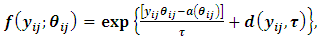(1)

where and are functions defined according to the chosen distribution of exponential family and is called the natural parameter of the distribution. For simplification we assume a balanced design, that is Let where are complete, observed and missing outcomes vectors of subject i respectively. Assuming that we have missing values for each subject i, then and

The conditional distribution of given the random effects has a GLM form and follows the exponential family form as in Eq. (1) with a canonical identity link function, i.e., Thus can be written in the form: 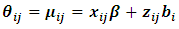, where is the jth row of the design matrix, for vector of fixed effect parameters and is the jth row in the design matrix of ith subject's random effect, The scale parameter is and

The GLMM can be written in the following form:

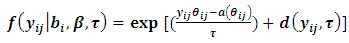(2)

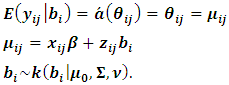(3)

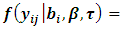
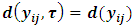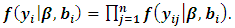
We assume that the scale parameter is constant and equals to one. Hence we can write and in Eq. (2). The function k(.) is the density function of the random effects with non-central mean variance covariance matrix and degrees of freedom.

Note that the responses at all occasions j=1,...,n for any subject i are conditionally independent given the common random effect Thus, the likelihood for N subjects with complete data can be written as follows:

(4)

The marginal likelihood of parameters is proportional to the marginal density function 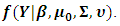This can be obtained by integrating out the random effect, i.e.

(5)

The integration in Eq. (5) is of high dimension (N x q). Thus evaluating the likelihood is cumbersome even with complete data. Moreover, in most cases this integration is intractable, specially, when the normality assumption is violated.

When the missing data mechanism is nonignorable, it is required to incorporate the parametric model for the missingness mechanism into the log-likelihood of complete data. Let the random vector be the missing data mechanism indicator whose jth component equals to 1 when the response is missing, otherwise it equals to zero. Under the selection model [19], the distribution of given the response is indexed with a parameter vector and has a multi-nominal distribution with cell probabilities, i.e.

(6)

Thus, the complete density for subject i is denoted by

(7)

where

The classical normality assumption of the random effects is not always realistic. The t-distribution offers a more viable alternative with respect to real-world data. Assuming a central multivariate t-distribution for the random effect, the density function k(.) is of the form

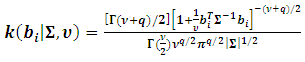(8)

The degrees of freedom is assumed to be known or unknown.

From Eq. (7), the complete-data log-likelihood can be defined as:

(9)

where is the set of all parameters.

3. Likelihood Estimation

In this section, the fixed effect parameters, the random effects parameters, and the missing data model's parameters, are estimated. A monotone pattern of missing data for the outcome variable is assumed, where The random effects of the ith subject, are unobserved, so they are also considered as missing data. Thus, in E-step of EM algorithm we need to integrate the complete-data log-likelihood in Eq. (9) over the missing data and In other words, in the E step the expectation of the log-likelihood function of complete data given the observed data and current estimate of parameters is obtained. The expectation is with respect to the joint distribution of missing data and . Starting with initial values the (t+1)th iteration of the EM algorithm proceeds as follows:

Ÿ The E-step: Obtain the expectations with respect to the conditional distribution of given in items 1 and 2 below. Also, obtain the conditional expectation with respect to conditional distribution of given in item 3 below.

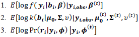Ÿ The M step: Find the values that maximize the function in item 1 above. Also, the values 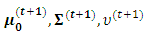that maximize the function in item 2 above and that maximize the function in item 3 above.

If convergence is achieved, the current values are the maximum likelihood estimates. Otherwise, let and return to the E-step.

The expectation of the log-likelihood for the ith subject at iteration (t+1) is

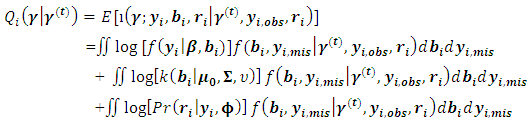(10)

where is the conditional distribution of missing data given the observed data and the current parameter estimates. The integral in Eq. (10) is intractable. Therefore, expectations are obtained via Monte Carlo simulation where sampling from is required.

The following two relations describe the complete conditional distributions

(12)

(13)

Sampling from the first complete conditional distribution in Eq. (11) is equivalent to sampling from because the missingness mechanism doesn't depend on the random effects. A single draw for the first dropout of the ith subject is generated from the predictive distribution instead of where are the current parameter estimates. Then an accept-reject sampling procedure is used to sample For more details, interested readers are referred to [20]. From properties of a multivariate normal, 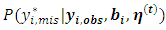is a normal distribution with mean and covariance matrix where

(13)

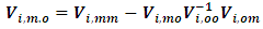(14)

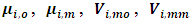
The and are suitable partitions from mean and covariance matrix V respectively.

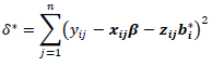
Sampling from the second complete conditional distribution in Eq. (12) is conducted using the Metropolis algorithm. A candidate value is generated from a proposal distribution which is chosen to be the density function of the random effects (the multivariate t). The generated value is accepted as opposed to keep the previous value with the probability:

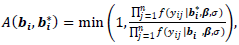(15)

where is a univariate normal and could be easily evaluated. The acceptance probability can be simplified as

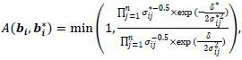(16)

where

and

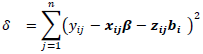The is jth row of and is the jth row in matrix of dimension and is the jth row in matrix of dimension

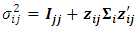(17)

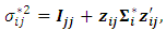(18)

where I is an identity matrix of dimension and is the variance covariance matrix of random effects component of dimension

Table 1. Parameter Estimates and their Corresponding Standard Errors (simulation study)

4. Simulation Study

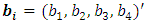
The aim of this simulation study is to evaluate the performance of the proposed techniques in Section (3). The number of subjects is assumed to be N = 30 subjects. The number of time points is assumed to be m = 7 time points. These numbers are chosen arbitrary for the sake of time. Hence, the response values are i = 1,2,…, 30, j=1,2,…,7. The random effects i = 1,2,…, 30, were generated from the multivariate t-distribution with dimension q =4 and known degrees of freedom The response values were generated, conditionally on the random effect, with variance covariance matrix which is assumed to have a first order autoregressive correlation structure AR(1).

The responses of the ith are modeled using the GLMM as

(19)

where is a subject random effects. The is a vector of ones The noise component follows a multivariate normal . The k=1,2,3; i=1,2,...,N; j=1,2,…,m are covariates (design matrix) associated with each subject. The values of are chosen as follows:

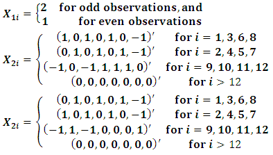The missing data process is modeled as a logistic model, where the missing data mechanism depends on the current and previous outcome as:

(12)

It is assumed that for all i. Also, are assumed to be independent for all (i,j) given and From Eq. (6) the missing data model for all observations can be written as:

(21)

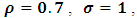
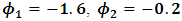
where is the occasion at the first dropout for subject i.

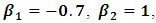
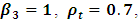
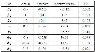
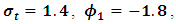
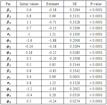
The parameter values are fixed as and

Table 1 shows the maximum likelihood estimates obtained using the MCEM algorithm, and the corresponding standard errors. 3000 samples were generated from missing data (missing outcome and random effect) with a burn-in period 500 iterations. Percentage of complete subjects is around 50%. As can be seen from Table 1, all parameters estimates are highly significant. All parameter estimates do not exceed a relative bias of 30% except its bias percentage is 43.14%, where the relative bias is defined as the ratio of bias with respect to actual values. Small values for standard errors show that we have good results, which are lying in confidence interval 95%.

All parameters of missing mechanism are significant, while parameter estimates of missing-mechanism for previous and current outcome are very significant, which support that the missing data-mechanism is non-ignorable.

5. Breast Cancer Data

This data set is related to quality of life among premenopausal women diagnosed with breast cancer. It is prepared via a clinical trail taken by the International Breast Cancer Study Group (IBCSG) [21]. The patients are followed for death, relapse and quality of life. The patients were randomized to one of four chemotherapy regimes. The patients were asked to answer a quality of life questionnaire at baseline (before starting treatment) and every three months for fifteen months. Therefore, each questionnaire should be answered 6 times in the specified period.

Table 2. Fixed parameters estimates and standard errors at different initial values (breast cancer data)

One of the effective determinants of quality of life was the Perceived Adjustment to Chronic Illness Scale (PACIS). This measures the amount of efforts the patient could bear to cope with her illness. The larger the score of the measure the greater the effort is done by patient to cope with her illness. It has a continuous scale from 0 as a best quality of life to 100 as the worst one. Assessment has been established for patients who remained alive during the study, so the missing data is not due to the death. Ten patients were died within the period are excluded from the study. Four hundreds and forty six patients have survived the period. Also, 64 cases have been removed as their missing responses were at first assessment. Thus, the number of patients in the trial is 382 subjects. A patient may refuse to answer the questionnaire on occasion and she is asked to answer the questionnaire in the next follow-up occasion. Therefore, the pattern of missingness in the trial is a combination of dropout and intermittent. The patient may refuse to answer the questionnaire, if her mood is poor, so the missingness mechanism is nonrandom. The percentage of complete subjects is 23%. Regarding the missing data, the percentage of patients with dropout pattern is 63%, while the percentage with intermittent pattern is 37%.

These data have been used in previous researches as follows: the first 9 months of the study were analyzed with only complete responses (complete case analysis) by [21]. An analysis for the first 6 months, taking into consideration the missing data, has been conducted by [22]. [11] have analysed the patient's self mood for 18 months of the study. They used normal random effects model with AR(1) covariance structure and logistic model for missing data mechanism. [24] used both AR(1) and unstructured covariance structure with hybrid pattern of missing data (intermittent and dropout missing).

In this paper, we assume a central multivariate t with known degrees of freedom (assumed to be 4) with dropout pattern of missing and AR(1) covariance structure. The intermittent missing values have been deleted, therefore, the number of patients in the trail becomes 284 patients. Also, following [21] a square root transformation for assessments is used to normalize data. A GLMM model is used to link the response variable to the treatments and the random effects with i = 1,2,…, 284, j =1,2,… 6 and treatments are defined as follows:

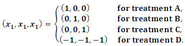The MCEM is implemented using 3000 samples with a bur-in period of 500 iterations.

Table 3. Parameters estimates and standard errors at different initial values (breast cancer data)

The proposed algorithm is implemented using several starting values of the parameters. The maximum likelihood estimates of the parameters are presented in Tables 2 where only different starting points are used for fixed effect parameters. The starting points were and The estimates of and were around 0.99, 1.21, -1.90, 0.26, and -0.24 respectively. The results in Table 3 are the maximum likelihood estimates using different starting points for all parameters.

Results show that the algorithm converges properly as the parameter estimates are similar for the different starting values. Also, all estimates are highly significant. Highly significant coefficients of treatments are indication of strong relationship between the response variable (PACIS) and the treatments. Given, that any patient receives only one treatment during the trail, the higher doze from treatment A or D, the smaller PACIS value i.e. a better quality of life the patient gets. On the other hand, the higher doze from treatment B or C, the higher PACIS value, i.e. patient endure hardship to cope with her life. Also, the significance of and supports that the missing data mechanism is non-ignorable.

6. Discussion

In this paper, a Monte Carlo EM algorithm is proposed to estimate the likelihood parameters of a longitudinal model in GLMM framework. We used a selection model for longitudinal data with non-ignorable missing mechanism in the context of dropout pattern. In this case the obtained likelihood function is intractable and it is difficult to integrate over the missing data (random effect and missing values of outcomes). Therefore a Monte Carlo EM algorithm is implemented. In the context of the proposed model, direct simulation is not possible because there is no defined mathematical form for the joint density of missing data (random effect and missing outcomes) given the observed data and current estimate of parameters. Thus, Monte Carlo Sampling techniques are used; Metropolis-Hastings and reject-accept techniques. Hessian matrix is used to estimate standard errors. The proposed algorithm is validated using a simulation study. Also, the proposed algorithm is applied to a real data set of breast cancer.