1. Introduction

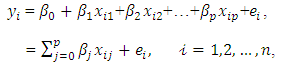
Regression analysis is a statistical tool that is useful in all areas of sciences. The objective of linear regression analysis is to study how a dependent variable is linearly related to a set of explanatory variables. The linear regression model is given by

(1)

where n is the number of observations, is the number of explanatory variables , and . The denotes the observed response, the represents the observation of the explanatory variable , denote the regression coefficients, and represents the random error (Birkes and Dodge, 1993). On the basis of the estimated parameters it is possible to fit the dependent variable as , and the estimates of the residuals for . In matrix notation the model can be written as .

The objective of regression analysis is to find the estimates of the unknown parameters, . One method of obtaining the estimates of is the method of least squares, which minimizes the sum of squared distances of all the points from the actual observation to the regression surface (Fox, 1997). Therefore, the objective is to find those values of that lead to the minimum value of .

(2)

The estimates are unbiased if . Among the class of linear unbiased estimators for , the estimator is the best in the sense that the variance of is the minimum, 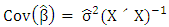, where is the mean square 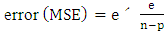. For this reason the least squares estimates are the best linear unbiased estimators, referred to as BLUE.

In order to use regression correctly, the assumptions on which it is based need to be met. The assumptions of the OLS are that the errors are normally distributed, have equal variance at all levels of the independent variables (homoscedasticity), and are uncorrelated with both the independent variables and with each other. It is also assumed that the variables are measured without error. When the assumptions are met, model inferences such as confidence intervals and hypothesis testing are very powerful.

A common problem in regression analysis is the presence of outliers. As defined by Barnett and Lewis (1994), outliers are observations that appear inconsistent with the rest of data. The outliers may occur as a result of unusual but explainable events, such as faulty measurement, incorrect recording of data, failure of a measurement instrument, etc. Each different reason may require different treatment. Heavy-tailed distributions usually generate outliers, and these outliers may have a marked influence on parameter estimates (Chatterjee and Hadi, 1986). Rousseeuw and Leroy (1987) classified outliers as vertical outliers, good leverage points and bad leverage points. Vertical outliers are those observations have outlying values for the corresponding error term (on the y-direction) but are not outlying in the space of explanatory variables (the x-dimension). Good leverage points are those observations that are outlying in the space of explanatory variables but that are located close to the regression line. Bad leverage points are those observations that are both outlying in the space of explanatory variables and located far from the true regression line. There are outliers in both the directions (x, direction of the explanatory variables and y, direction of the response variable).

The aim of this paper is to compare the robust methods of estimation of regression parameters. This is specific to the outliers in y-direction. The comparison is conducted via simulation study and a real application. The paper is organized as follows. Section 2 is devoted to the evaluation and comparison criteria of regression estimators. In Section 3 we review the robust regression methods that achieve high breakdown point, high efficiency or both. Section 4 is devoted for the simulation study and Section 5 for the real application. In Section 6 we conclude the paper.

2. Evaluating Regression Estimators

The regression estimators can be evaluated and compared using different criteria. Although some criteria are more important than others, for a particular type of datasets, the ideal estimator would have positive characteristics of all criteria. These criteria include the following.

2.1. The Breakdown Point

The breakdown is the degree of robustness of an estimate in the presence of outliers (Hampel, 1974). The smallest possible breakdown point is 1/n which tends to 0% when the sample size n becomes large. This is the case in the least squares estimators. If a robust estimator has a 50% breakdown point then 50% of the data could contain outliers and the coefficients would remain useable.

One aim of robust estimators is a high finite sample breakdown point . A formal finite sample definition of breakdown is given in Rousseeuw and Leroy (1987). Using a sample of n data points such that and let T be a regression estimator. Applying T to the sample Z yields the regression estimator T(Z) = . Consider all possible corrupted samples obtained by replacing the data points by the arbitrary values which allows for very bad outliers. The maximum bias that can be caused by this contamination is

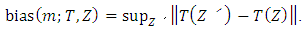(3)

If the is infinite, then the m outliers can have an arbitrarily large effect on T, which may be expressed by saving that estimator breaks down. Thus, the finite sample breakdown point of the estimator at the sample of Z is defined as:

(4)

2.2. The Mean Square Errors (MSE)

One of the performance criteria used to evaluate techniques (methods) of regression is the mean square errors which is given by

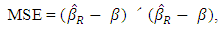(5)

where is a vector of robust parameter estimates and is the vector of the true model coefficients.

2.3. The Bounded Influence

Bounded influence in the X-space is the estimator’s resistance to being pulled towards the extreme observations in the X-space. Determining whether or not an estimator has a bounded influence is obtained by a study of the influence function. As defined by Seber (1977) influence function (IF) is a measure of the rate at which the estimator (T) responds to a small amount of contamination on x.

Hampel (1968, 1974) defined the influence function of the estimator T, at the underlying probability distribution, F, by

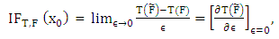(6)

where denotes the estimator of interest, expressed as a functional. The functional represent the estimator of interest under this altered c.d.f.. Thus, the influence function is actually a first derivative of an estimator, viewed as functional, and measures the influence of the point on the estimator T.

3. Robust Regression Methods

Many robust methods have been proposed in literature to achieve high breakdown point, high efficiency or both. Therefore, robust regression methods can be divided into three broad categories: high-breakdown point estimators, high efficiency estimators and multiple property estimators (related classes of efficient high-breakdown estimators). Each category contains a class of estimators derived under similar conditions and with comparable theoretical statistical properties.

3.1. High-Breakdown Point Estimators

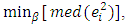
High-breakdown point (HBP) regression estimators, also known as resistant estimators, can achieve up to a 50% breakdown point. They are useful for outliers detection and initial estimators. However, these estimators have low efficiency and unbounded influence. Due to this fact these estimators cannot be used as stand-alone estimators. The common estimators of this type are outlined in the following lines.

The repeated median (RM) estimator

Siegel and Benson (1982) propose the repeated median (RM) estimator with a 50% breakdown point. For any p observations 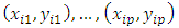the repeated median estimator determines a unique parameter vector which is defined as

(7)

The RM estimator is not affine equivariant. It was applied to a biological problem by Siegel and Benson (1982).

The least median squares (LMS) estimator

Rousseeuw (1984) propose the least median of squares (LMS) estimator. This approach can be thought of as being similar to the ordinary least squares, except that the median value is used instead of the mean value. The LMS estimator can be expressed as:

(8)

where "med" denotes the median. The breakdown point of LMS is 50%. Therefore, it resists the effect of outliers even when they comprise nearly half of the data. The LMS lacks efficiency under normality although it is highly robust. The LMS can be robust with respect to outliers in both the x and the y directions but does not contain an influence function that is theoretically, bounded in the x-space. It satisfies all three equivariance properties; regression equivariance, scale equivariance, and affine equivariance (Rousseeuw and Leroy, 1987).

The least trimmed squares (LTS) estimator

Rousseeuw (1984) propose the least trimmed of squares (LTS) estimator as a high efficiency alternative to the LMS. The LTS is defined as

(9)

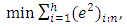
where are the ordered squared residuals from the smallest to the largest. Rousseeuw and Leroy (1987) recommend using , where is the trimmed percentage.

Rousseeuw and van Driessen (2006) propose that the LMS estimator should be replaced by the least trimmed squares (LTS) estimator for large data sets. The best robustness properties are achieved when h is approximately n/2. In this case the breakdown point attains 50% (Rousseeuw and Leroy, 1987). The breakdown point of the LMS and the LTS are equal if . The LTS has convergence rate and it converges at a rate similar to the M-estimators (Rousseeuw, 1984). Zaman et al. (2001) mention that although the LTS method is good at finding out the outliers, it may sometimes eliminate too many observations and this may not give the true regression relation about the data. The LTS estimator is regression, scale, and affine equivariant (Rousseeuw and Leroy, 1987). The LTS-estimator statistical efficiency is better than the LMS, with higher asymptotic Gaussian efficiency of 7.1% (Rousseeuw and van Driessen, 2006).

The least Winsorized squares (LWS) estimator

Another alternative method to the LS estimation procedure is the Winsorized regression which is applied by altering the data values based upon the magnitude of the residuals (Yale and Forsythe, 1976). The aim of Winsorization is to diminish the effect of contamination on the estimators by reducing the effect of outliers in the sample. The estimator is given as:

(10)

where h may depend on some fraction a. For simple linear regression, Winsorization is applied by ordering the values and modifying extreme Y-values, in an iterative fashion, by replacing the observed residual for an extreme Y -value with the next closest (and smaller) residual in the dataset, and, then, computing new Y -values using the formulation for an observed score as presented above. These new Y-values are used to compute new slope and intercept estimates for the regression line, and then a new set of residuals is obtained. The process of estimation, obtaining residuals, and data modification are continued for a specified number of iterations (Yale and Forsythe, 1976; Nevitt and Tam, 1998). The LWS is regression, scale, and affine equivariant similar to the LMS and the LTS (Rousseeuw and Leroy, 1987). Its breakdown is 50% when h is approximately n/2 (Rousseeuw and Leroy, 1987).

The S-Estimator

Rousseeuw and Yohai (1984) develop a high-breakdown estimator that minimizes the dispersion of the residuals. The S –estimator is defined by

(11)

with final scale estimate

(12)

where is the residual for candidate . The dispersions are defined as the solution of the equation:

(13)

The constant may be defined as or to ensure that the S-estimator of the residual scale is consistent for whenever it is assumed that the error distribution is normal with zero mean and variance, where is the standard normal distribution. The function must satisfy the following conditions:

1. is symmetric, continuously differentiable and .

2. There exists the constant such that is strictly increasing on and constant on .

The term S-estimator is used to describe the class of robust estimation because it is derived from a scale statistic in an implicit way. For one often chooses the function

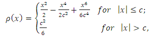(14)

where c is an appropriate tuning constant (Rousseeuw and Yohai, 1984). The derivative of this function is known as Tukey’s biweight function:

(15)

In general, will always be zero for because of condition 2; such functions are usually called “re-descending” (Rousseeuw and Yohai, 1984). The breakdown point of the S-estimator can be 50%, assuming a condition is satisfied relating the constant with the function such that .

The S-estimator is regression, scale, and affine equivariant. It is also asymptotically normal with rate of convergence. Efficiency of the S-estimators can be increased at the expense of decreases in breakdown point (Rousseeuw and Leory, 1987). The S-estimator perform marginally better than the LMS and the LTS because the S-estimator can be used either as a high breakdown initial estimate with a high efficiency, or as a moderate breakdown (25%), moderate efficiency (75.9%) estimator (Rousseeuw and Leroy, 1987).

3.2. Efficiency Estimators

An efficient estimator provides parameter estimates close to those from an the OLS (the best linear unbiased estimator) which fits in an uncontaminated sample NID error terms. While the common efficient techniques are not high breakdown nor bounded-influence.

The norm or Least Absolute Deviations (LAD) Estimator

Boscovich introduced the method of least absolute deviations (LAD) in 1757, almost 50 years before the method of least squares was discovered by Legendre in France around 1805 (Birkes and Dodge, 1993). The least absolute deviations (LAD), also known as least absolute errors (LAE), the least absolute value (LAV) or the regression, is a mathematical optimization technique similar to the popular least squares technique in the attempts to find a function which closely approximates a set of data. (Cankaya, 2009).

In the LAD method, the coefficients are chosen so that the sum of the absolute deviations of the residuals is minimized as:

(16)

The LAD method is especially suitable when it is believed that the distribution of the errors has very heavy tails or is asymmetric or when the sample is very large. Because the LAD estimates have relatively low variance in the case of a heavy tailed error distribution, they have low bias in the case of an asymmetric error distribution and any reasonable estimate has low variance and control bias in the case of large samples (Birkes and Dodge, 1993). The LAD reduces the effects of outliers among the Y values but it does not protect against outliers among the X values (leverage points), which have a large effect on the model fit. Hence, it is a robust with respect to outliers in the y-direction and it is not robust with respect to the x-outliers (Wilcox, 2010). The breakdown point of the LAV is 1/n. Thus the effect of one x-axis data outlier will change the regression line, causing the line to pass through the outlying data point.

The M-estimator (M)

Huber introduced in 1973 the idea of M-estimation as an alternative robust regression estimator to the least squares. The class of M-estimator models contains all models that are derived to be maximum likelihood models. The M-estimate is nearly as efficient as the OLS. This method is based on the idea of replacing the sum of squared residuals used in the LS estimation by another function of residuals, .

(17)

The function gives the contribution of each residual to the objective function. A reasonable should posses the following properties: ; (non-negativity); 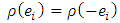(symmetric); 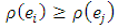for (monotonicity or non-decreasing function of and is continuous ( is differentiable). Because the M- estimator is not scale invariant the minimization problem is modified by dividing the function by a robust estimate of scale s, so the formula becomes

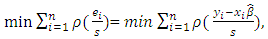(18)

where s is a robust estimate of scale. A popular choice for s is the median absolute deviation

The least squares estimator is a special case of the function where . The system of normal equations to solve this minimization problem is found by taking partial derivatives with respect to and setting them equal to 0, yielding 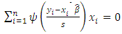, where is the derivative of . In general, the function is nonlinear and formula (18) must be solved by iterative methods. While several nonlinear optimization techniques could be employed, iteratively reweighted least squares (IRLS) is most widely used in practice and it is the only one considered for this research. The M-estimators can almost equivalently be described by a function (posing a minimization problem) or by its derivative, an function (yielding a set of implicit equation(s)), which is proportional to the influence function. Robust regression procedures can be classified by the behavior of their function. The key to M- estimation is finding a good function.

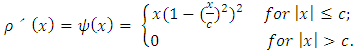
Although there are many specific proposals for the -function, they can all be grouped into one of two classes: monotone and redescending. A monotone -function (e.g. Huber’s estimator) does not weight large outliers as much as least squares. The -function of Huber estimator is constant-linearly increasing-constant. A re-descending -function (e.g. Hample’s and. Ramsay’s) increases the weight assigned to an outlier until a specified distance and then decreases the weight to 0 as the outlying distance gets larger. Montgomery et al. (2012) introduce two types of a re-descending -function: soft re-descender and hard re-descender. Alamgir et al. (2013) propose a new re-descending M-estimator, called Alamgir re-descending M-estimator abbreviated as (ALARM). The -function of ALARM estimator is defined as

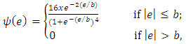(19)

where e denotes the error and b is a tuning constant. However, the M-estimators are not robust to x-axis outliers; therefore, their breakdown point is 1/n because of the effect of a single outlying observation. The M-estimators are statistically more efficient than L₁ at a central model with Gaussin errors (Rousseeuw and Yohai, 1984). Its asymptotic relative efficiency with respect to least squares is at least 0.81 (Birkes and Dodge, 1993). For regression analysis, some of the re-descending M-estimators can attain the maximum breakdown point. Moreover, some of them are the solutions of the problem of maximizing the efficiency under bounded influence function when the regression coefficient and the scale parameter are estimated simultaneously. Hence re-descending M-estimators satisfy several outlier robustness properties (Muthukrishnan and Radha, 2010).

3.3. Multiple Property Estimators (Related classes of efficient high breakdown estimators)

The discussion of robust estimators has clearly shown that no estimator has all the desirable properties. The multiple property estimators have been proposed to combine several properties into a single estimator.

The multi-stage (MM) estimator

Yohai (1987) introduces the multi-stage estimator (MM-estimator), which combines high breakdown with high efficiency. The MM-estimator is obtained using a three-stage procedure. In the first stage, an initial consistent estimate with high breakdown point but possibly low normal efficiency is obtained. Yohai (1987) suggests using the S-estimator for this stage. In the second stage, a robust M-estimator of scale parameter of the residuals based on the initial value is obtained. In the third stage, an M-estimator starting at is obtained.

In practice, the LMS or S-estimate with Huber or bi-square functions is typically used as the initial estimate . Let and assume that each of the functions is bounded, i = 0 and 1. The scale estimate satisfies the following equation:

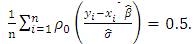(20)

If the function is biweight, then ensures that the estimator has the asymptotic BP = 0.5. Although the MM-estimators have a high breakdown and are efficient, they do not necessarily have bounded influence, meaning that they may not perform especially well in the presence of high leverage points.

The estimator

Yohai and Zamar (1988) introduce a new class of robust estimators; the estimator. The estimator has, simultaneously, the following properties: i) they are qualitatively robust, ii) their breakdown point is 0.5, and iii) they are highly efficient for regression models with normal errors.

In the estimator, the coefficients are chosen so that a new estimator of the scale of the residuals is minimized as:

(21)

where the scale is given by

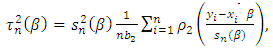(22)

with is the M-estimator of scale that satisfies the solution

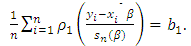(23)

The functions are assumed to be symmetric, continuously differentiable bounded, strictly increasing on , and constant on with

The parameters and are tuned to obtain consistency for the scale at the normal error model:

(24)

where is the standard normal distribution. Like the MM-estimators, the estimators have the breakdown point of an S-estimator based on the loss function , while its efficiency is determined by the function which is used in Eq. (18) (Yohai and Zamar, 1988). The estimators possess theoretical advantages over the MM-estimators: they are associated with a robust and efficient scale estimate (Barrera et al., 2008).

The robust and efficiency weighted least squares (REWLSE) estimator

Gervini and Yohai (2002) introduce a new class of estimators that simultaneously attain the maximum breakdown point and full asymptotic efficiency under normal errors. They weight the least squares estimators with adaptively computed weights using the empirical distribution of the residuals of an initial robust estimator.

Consider a pair of initial robust estimators of parameters and scale and respectively. If , the standardized residuals are defined as:

(25)

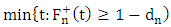A large value of would suggest that is an outlier. In order to maintain the breakdown point value of the initial estimator and to have a high efficiency, they proposed the use of an adapted cut-off value, , as where is the empirical cumulative distribution function of the standardized absolute residuals and is the measure of the proportion of the outliers in the sample. The values of are given as

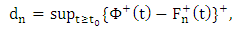(26)

where denotes the normal cumulative distribution of the random errors, is the initial cut-off value and denotes the positive part between and . The form of the weights, W, and the REWLS estimator, , are defined as

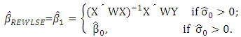(27)

The weight function, W, is chosen in order to have a hard-rejection to outliers

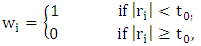(28)

.

Note that with these weights, estimator maintains the same breakdown point value of the initial estimator . Touati et al. (2010) modify the robust estimator of Gervini and Yohai (2002) and labeled it as the Robust and Efficient Weighted Least Squares Estimator (REWLSE), which simultaneously combines high statistical efficiency and high breakdown point by replacing the weight function by a new weight function.

4. Simulation Study

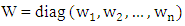
A simulation study is conducted to compare different methods of estimation. These methods are:

1. The ordinary least squares estimator (OLS);

2. The least median squares estimator (LMS);

3. The least trimmed squares estimator (LTS);

4. The S-estimator (S);

5. The least absolute value estimator (LAV);

6. The M-estimator; the Huber's M-estimator (M_Huber) with b=1.345;

7. The Tukey's M-estimator (M_Tukey) with k₁ = 4.685; and

8. The Hampel's M-estimators (M_Hampel) with a=1.7, b=3.4, and c=8.5;

9. The MM-estimators (MM) using bi-square weights and k₁ =4.685, and

10. The robust and efficiency weighted least squares estimator (RWLSE).

The comparison criteria are the mean squares error (MSE), total mean squares error (TMSE), absolute bias (AB) and total absolute bias (TAB) of the estimates of the regression coefficients.

The data are generated according to the multiple linear regression model:

where and the are independent. The true value of the regression parameters are all equal one; . The data simulation is repeated 5000 times to obtain 5000 independent samples of Y and X of a given size n. The used sample sizes are n = 30 and n = 100. Comparisons of the properties of some robust methods are based on outliers in the y-direction (response direction). In order to cover the effects of various situations on the regression coefficients, seven scenarios of the density function of the errors (e) have been used. These scenarios are:

Scenario I: e ~ N (0, 1); the standard normal distribution.

Scenario II: e ~ t-distribution with df = 1; the t-distribution with degrees of freedom 1 (Cauchy distribution).

Scenario III: e ~ t-distribution with df = 5; the t-distribution with degrees of freedom 5.

Scenario IV: e ~ slash (0, 1); the slash distribution denoted by N (0, 1)/U (0, 1).

Scenario V: e ~ N (0, 1) with 20% outliers in y-direction generated from N (0, 10).

Scenario VI: e ~ N (0, 1) with 40% outliers in y-direction generated from N (0, 10).

Scenario VII: e ~ 0.80*N(0,1) + 0.20*N(0,10); contaminated mixture of normal.

For each scenario the mean square error (MSE), the total mean square error (TMSE), the absolute bias (AB) and the total absolute bias (TAB) have been obtained using the OLS-estimator, the LTS-estimator, the LMS-estimator, the S-estimator, the LAV-estimator, the M-estimators, the MM-estimator and the REWLSE. The results are not displayed for the sake of parsimony, however the following conclusions can be drawn.

Scenario I: the OLS estimate achieves the best performance. The decline in the performance of the other estimates compared to the performance of the OLS-estimate is the price paid by the methods due to the existence of outliers. The M-estimate, the MM-estimate, the REWLSE, and the LAV-estimate have better performance comparable to the estimates, as well as they provide a performance equal to the performance of the OLS-estimate. The performance of the high breakdown point estimates are poor compared to the OLS-estimate, the M-estimate, the LAV-estimate, the MM-estimate, or the REWLSE. As the sample size increases, the value of both the TMSE and the TAB decrease.

Scenario II: The OLS estimates give the worst result with regard to the TAB and the TMSE. The M_Tukey -estimate, the MM-estimate, the LAV-estimate, the REWLSE and the S-estimate tend to give lower TMSE and TAB values than other robust estimators. The LMS estimate and the LTS estimate have higher TMSE and TAB values than other robust estimators.

Scenario III: The OLS estimates give the highest TMSE and TAB values. The M_Huber estimates and the MM-estimates tend to give smaller TMSE and TAB values than the others. The LMS-estimates, the LTS estimates and the S-estimates have higher TMSE and TAB values. If the errors follow the t-distribution, the TMSE and TAB of each estimate decreases as the degrees of freedom (df) increases.

Scenario IV: The OLS estimates have the largest TMSE and TAB values. The M_Tukey estimate and the MM-estimates tend to give smaller TMSE and TAB than others. The LMS estimates and the LTS-estimates tend to give a higher TMSE and TAB than others.

Scenario V: It is noticed that when the data contain 20% outliers from the N (0, 10) in the y-direction, the OLS-estimate has the largest TMSE and TAB. The REWLSE, the M_Tukey estimator and the MM-estimator, tend to give a lower TMSE and TAB than others.

Scenario VI: We can see that when the data contain 40% outliers from N (0, 10) in the y-direction, the OLS estimator decline in performance, while most of the other estimators are have good performances depending on the percentage and direction of contaminations. In general, the TMSE and TAB values decrease when the sample sizes increase while the TMSE and TAB values increase as the proportion of contaminations "outliers" increases.

Scenario VII: The OLS estimator has the largest TMSE and TAB values. The REWLSE, the M_Tukey estimator and the MM-estimator tend to give lower TMSE and TAB values than other robust estimators. The LMS-estimator and the LTS estimator achieve higher TMSE and TAB values than other robust estimators.

5. Application

A real data set (growth data) given by De Long and Summers (1991) is used. The aim is to evaluate the performance of various estimators. This data set measures the national growth of 61 countries from all over the world from the years 1960 to 1985. The data set contains many variables. They are the GDP growth per worker (GDP) which the response variable, the labor force growth (LFG), the relative GDP gap (GAP), the equipment investment (EQP), and non-equipment investment (NEQ). The main claim is that there is a strong and clear relationship between equipment investment and productivity growth. The regression equation they used:

(29)

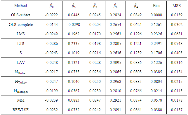
where and are regression parameters.

Zaman et al. (2001) note that the growth study of De Long and Summers suffers from the problem of outliers in the y-direction (response direction). Zaman et al. (2001) use robust regression techniques and show that the 60th country in the data is an outlier.

We compare the OLS estimator, the LMS-estimator, the LTS-estimator, the S-estimator, the LAV-estimator, the Huber's M-estimator, the Tukey's M-estimator, the Hampel's M-estimator, the MM-estimator and the REWLSE by using bias and Mean square error values.

The results of the estimated regression parameters for the ten methods with all data points (complete data) are presented in Table (1). Also, results of the OLS method are displayed for the 60 data point (subset) ignoring the outlier; Zambia. The value of the bias and the MSE for the OLS estimate change from 0.1261 and 0.0302 (complete data) to 0 and 0.0139 (subset data). Thus, it is clear that the outlier strongly influences the OLS estimate. High-breakdown estimates (the LTS estimate, the LMS estimate, and the S-estimate) have low performance when the contamination is in the direction of the response variable only. The LAV estimate also has poor performance in this real data example.

Depending on the bias we can conclude that the Hampel's M-estimate and the REWLSE perform better than the others. When the MSE is considered, it indicates that the Hampel's M-estimate and the Huber's M-estimate perform better than the others.

Table (1). Estimates of regression coefficients, the bias and the MSE for growth data

6. Conclusions

The mean square errors (MSE) and the bias are of interest in regression analysis in presence of outliers. The performances of different estimates are studied using a simulation study and a real data for outliers in y-direction. The estimates of the regression coefficients using nine methods are compared with the ordinary least-squares. Depending on the simulation study the Tukey's M-estimator give a lowest TAB and TMSE values than others, for all sample sizes and when the contamination is in the y-direction. For the real data the Hampel's M-estimators gives lower bias and MSE values than others when the contamination is in the y-direction.

The work can be extended in future to handle outliers in x-direction; good leverage points. Another possible future direction is to compare robust methods when outliers are in both y-direction and x-direction (bad leverage points).

ACKNOWLEDGEMENTS

The authors would like to thank referees and editors for their help and constructive comments that improve significantly the manuscript.