1. Introduction

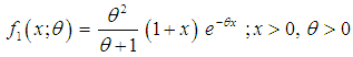
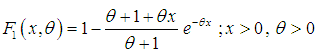
The modeling and statistical analysis of real lifetime data-sets from almost all applied sciences including engineering, biomedical science, insurance, finance, and demography, amongst others are crucial for policy makers and statistical literature is flooded with many lifetime distributions. The main reason for having many lifetime distributions is that each distribution is based on certain assumptions and a small change in their assumptions leads to a new distribution. A number of lifetime distributions for modeling lifetime data such as exponential, Lindley, Shanker, Akash, Aradhana, Sujatha, Amarendra, Devya, gamma, lognormal, and Weibull have been introduced in recent years in statistics literature. The exponential, Lindley, Shanker, Akash, Aradhana, Sujatha, Amarendra, Devya and the Weibull distributions have one important advantage over gamma and lognormal distributions is that the survival functions of the gamma and the lognormal distributions cannot be expressed in closed forms and both require numerical integration. Exponential, Lindley, Shanker, Akash, Aradhana, Sujatha, Amarendra and Devya distributions consists of one parameter and Lindley, Shanker, Akash, Aradhana, Sujatha, Amarendra and Devya distributions have advantage over exponential distribution that the exponential distribution has constant hazard rate whereas Lindley, Shanker, Akash, Aradhana, Sujatha, Amarendra and Devya distributions have monotonically increasing hazard rate. Further, the nature of Devya distribution is more flexible than exponential, Lindley, Shanker, Akash, Aradhana, Sujatha, and Amarendra distributions for modeling real lifetime data-sets from biomedical science and engineering.

The probability density function (p.d.f.) and the cumulative distribution function (c.d.f.) of Lindley distribution introduced by Lindley (1958) are given by

(1.1)

(1.2)

Ghitany et al (2008) have discussed various properties of this distribution and showed that (1.1) provides a better model for some applications than the exponential distribution. Shanker et al (2015) have detailed and critical comparative study of exponential and Lindley distributions for modeling various lifetime data and gave several examples to show the superiority of Lindley over exponential and that of exponential over Lindley. A number of researchers in distribution theory have worked on modifications, extension, generalizations, and mixture of Lindley distribution suiting their applications in different areas of knowledge including Sankaran (1970), Zakerzadeh and Dolati (2009), Nadarajah et al (2011), Deniz and Ojeda (2011), Bakouch et al (2012), Shanker and Mishra (2013 a, 2013 b, 2016), Shanker and Amanuel (2013), Shanker et al (2013), Elbatal et al (2013), Ghitany et al (2013), Merovci (2013), Ashour and Eltehiwy (2014), Oluyede and Yang (2014), Singh et al (2014), Sharma et al (2015), Alkarni (2015), Pararai et al (2015), Abouammoh et al (2015), Shanker and Hagos (2015), Shanker et al (2015, 2016 a, 2016 b, 2016 c), are some among others.

The probability density function (p.d.f.) and the cumulative distribution function (c.d.f.) of Shanker distribution introduced by Shanker (2015 a) are given by

(1.3)

(1.4)

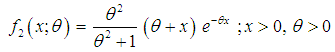
It was shown by Shanker (2015 a) that the density (1.3) is a two-component mixture of an exponential distribution and a gamma distribution with their mixing proportions and respectively. Shanker (2015 a) has discussed its various mathematical and statistical properties including its shape, moment generating function, moments, skewness, kurtosis, hazard rate function, mean residual life function, stochastic orderings, mean deviations, distribution of order statistics, Bonferroni and Lorenz curves, Renyi entropy measure, stress-strength reliability, some amongst others. It has been shown by Shanker (2015 a) that Shanker distribution gives better fit than exponential and Lindley distribution for modeling real lifetime data-sets. Shanker (2016 a) has obtained Poisson mixture of Shanker distribution named Poisson-Shanker distribution (PSD) and discussed its various mathematical and statistical properties, estimation of its parameter and applications for various count data-sets. Shanker and Hagos (2016 a, 2016 b) have obtained the size-biased and zero-truncated versions of Poisson-Shanker distribution (PSD), derived their interesting mathematical and statistical properties, discussed the estimation of their parameter and applications for count data-sets from different fields of knowledge.

The probability density function (p.d.f.) and the cumulative distribution function (c.d.f.) of Akash distribution introduced by Shanker (2015 b) are given by

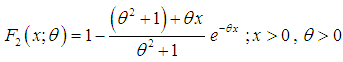
(1.5)

(1.6)

It was shown by Shanker (2015 b) that the density (1.5) is a two-component mixture of an exponential distribution and a gamma distribution with their mixing proportions and respectively. Shanker (2015 b) has discussed its various mathematical and statistical properties including its shape, moment generating function, moments, skewness, kurtosis, hazard rate function, mean residual life function, stochastic orderings, mean deviations, distribution of order statistics, Bonferroni and Lorenz curves, Renyi entropy measure, stress-strength reliability, some amongst others. Shanker et al (2016 c) has detailed and critical study about modeling and analyzing real lifetime data-sets from various fields of biomedical science and engineering using one parameter Akash, Lindley and exponential distributions and shown that in majority of data-sets Akash distribution gives better fit. Shanker (2016 b) has obtained Poisson mixture of Akash distribution named Poisson-Akash distribution (PAD) and discussed its important properties, estimation of its parameter and applications for various count data-sets. Further, Shanker (2016 c, 2016 d) has also obtained the size-biased and zero-truncated versions of PAD, derived their important mathematical and statistical properties, and discussed the estimation of parameter and applications for count-data-sets.

The probability density function (p.d.f.) and the cumulative distribution function (c.d.f.) of Aradhana distribution introduced by Shanker (2016 e) are given by

(1.7)

(1.8)

It was shown by Shanker (2016 e) that the density (1.7) is a a three-component mixture of an exponential distribution, a gamma distribution, and a gamma distribution with their mixing proportions , and , respectively. Shanker (2016 e) has discussed its important mathematical and statistical properties, estimation of parameter and applications for modeling various real lifetime data-sets and observed that Aradhana distribution gives better fit than exponential, Lindley, Shanker and Akash distributions. Shanker (2016 f) has obtained Poisson-Aradhana distribution (PAD), a Poisson-mixture of Aradhana distribution and showed that PAD gives a better fit than Poisson-distribution and Poisson-Lindley distribution (PLD) for modeling count data. Further, Shanker and Hagos (2016 c, 2016 d) have derived size-biased and zero-truncated versions of PAD and discussed their mathematical and statistical properties, estimation of their parameter using maximum likelihood estimation and method of moments and their applications.

The probability density function (p.d.f.) and the cumulative distribution function (c.d.f.) of Sujatha distribution introduced by Shanker (2016 g) are given by

(1.9)

(1.10)

It can be easily shown that the density (1.9) is a three-component mixture of an exponential distribution, a gamma distribution, and a gamma distribution with their mixing proportions , and respectively. Shanker (2016 g) has done a detailed study of its various properties, estimation of parameter and applications for modeling real lifetime data-sets and observed that it gives a better model for modeling real lifetime data-sets than exponential, Lindley, Shanker and Akash distributions. Shanker (2016 h) has also obtained a Poisson-mixture of Sujatha distribution and named it ‘Poisson-Sujatha distribution (PSD)’ and discussed its properties, estimation of parameter and applications. Shanker and Hagos (2016 e) has detailed study about applications of PSD for modeling various count data-sets from biological sciences. Further, Shanker and Hagos (2016 f, 2016 g) have obtained size-biased and zero-truncated versions of PSD and discussed their properties, estimation of their parameter and their applications in different fields of knowledge. In fact, Shanker and Hagos (2016 h) has detailed study about zero-truncation Poisson, Poisson-Lindley and Poisson-Sujatha distributions and their applications for modeling count data-sets from different fields of knowledge which are structurally excluding zero count.

The probability density function (p.d.f.) and the cumulative distribution function (c.d.f.) of Amarendra distribution introduced by Shanker (2016 i) are given by

(1.11)

(1.12)

Shanker (2016 i) has shown that the density (1.11) is a four - component mixture of exponentialdistribution, a gammadistribution, a gamma distribution and a gamma distribution with their mixing proportions,, , and respectively. Shanker (2016 i) has done a detailed study of its various properties, estimation of parameter and applications for modeling real lifetime data-sets from biomedical science and engineering and concluded that it gives better fit than exponential, Lindley, Shanker, Akash, Aradhana and Sujatha distributions. Shanker (2016 j) has also obtained a Poisson-mixture of Amarendra distribution and named it ‘Poisson-Amarendra distribution (PAD)’ and discussed its various properties, estimation of parameter and applications for count data-sets. Further, Shanker and Hagos (2016 i, 2016 j) have obtained size-biased and zero-truncated versions of PAD and discussed their properties, estimation of their parameter and applications in different fields of knowledge.

The Probability density function (p.d.f.) and the cumulative distribution function (c.d.f.) of Devya distribution proposed by Shanker (2016 k) are given by

(1.13)

(1.14)

Shanker (2016 k) has shown that the density (1.13) is a five - component mixture of a exponentialdistribution, a gamma distribution, a gamma distribution, a gamma distribution and a gamma distribution with their mixing proportions , , , , and respectively. Shanker (2016 k) has done a detailed study of some of its mathematical and statistical properties, estimation of its parameter and applications for modeling lifetime data from engineering and medical science and observed that it provides a better model than exponential, Lindley, Shanker, Akash, Aradhana, Sujatha, and Amarendra distribution for modeling real lifetime data-sets.

2. A New Lifetime Distribution

In this section a new lifetime distribution for modeling and analyzing real lifetime data-sets has been suggested. The Probability density function (p.d.f.) of the new one parameter lifetime distribution can be introduced by

(2.1)

We would name this new one parameter lifetime distribution, “Shambhu distribution”. The corresponding cumulative distribution function (c.d.f.) of Shambhu distribution can be obtained as

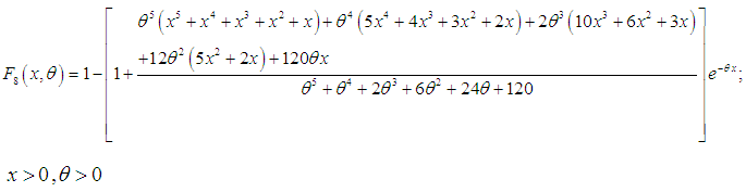(2.2)

It can be easily shown that Shambhu distribution is a six - component mixture of exponential distribution, a gammadistribution, a gamma distribution, a gamma distribution, a gamma distribution, and a gamma distribution with their mixing proportions , , , , , and respectively.

The graphs of the p.d.f. and the c.d.f. of Shambhu distribution for different values of θ are shown in figures 1(a) and 1(b)

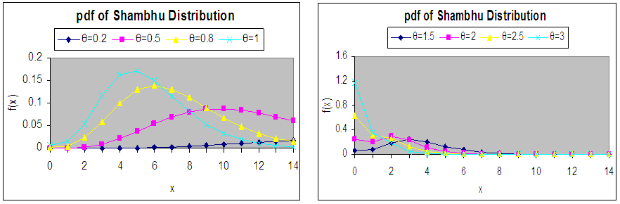Figure 1(a). Graphs of p.d.f. of Shambhu distribution for selected values of parameter θ

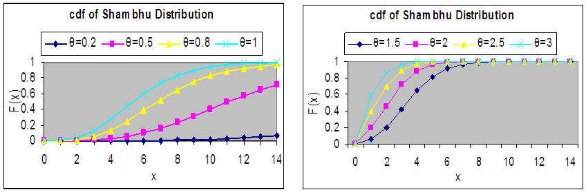Figure 1(b). Graphs of c.d.f. of Shambhu distribution for selected values of parameter θ

3. Statistical Properties

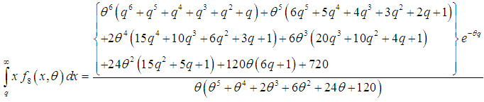
In this section, the basic statistical properties of Shambhu distribution including moment generating function, rth moment about origin, moments about origin, central moments, coefficient of variation, coefficient of skewness, coefficient of kurtosis and index of dispersion have been derived and discussed.

The moment generating function of Shambhu distribution (2.1) can be obtained as

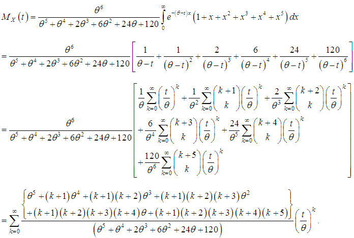The r the moment about origin of Shambhu distributon (2.1) can be obtained as

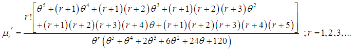The first four moments about origin of Shambhu distribution (2.1) are thus obtained as

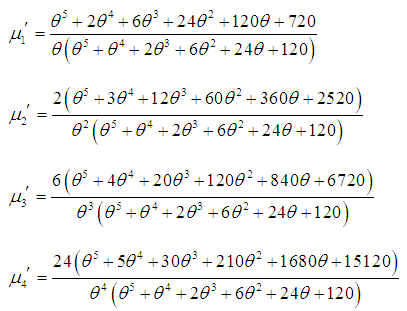Using the relationship between moments about mean and moments about origin, the moments about mean of Shambhu distribution (2.1) are obtained as

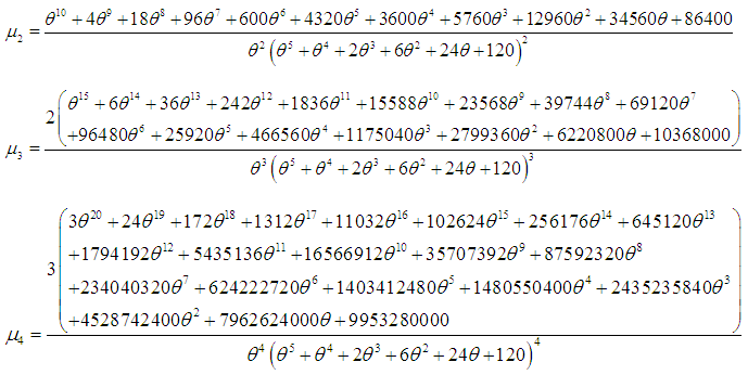The coefficient of variation, coefficient of skewness, coefficient of kurtosis, and index of dispersion of Shambhu distribution (2.1) are thus obtained as

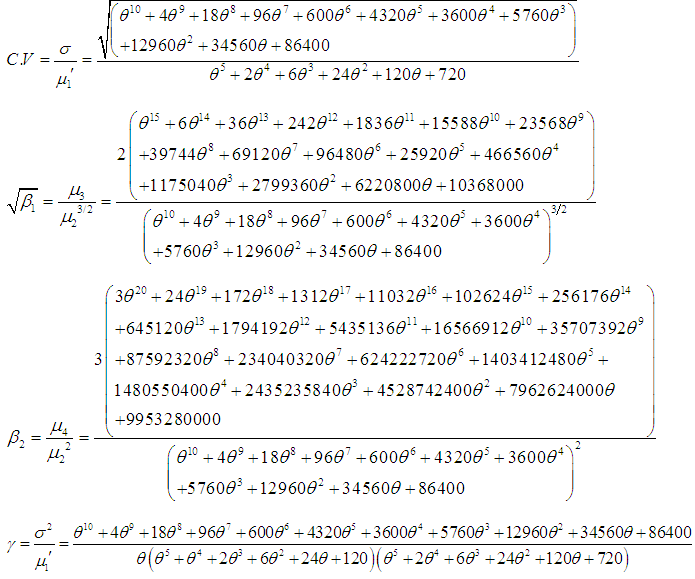The condition under which Shambhu distribution is over-dispersed, equi-dispersed, and under-dispersed has been given along with conditions under which Devya, Amarendra, Sujatha, Aradhana, Akash, Shanker, Lindley and exponential distributions are over-dispersed, equi-dispersed, and under-dispersed in table 1.

Table 1. Over-dispersion, equi-dispersion and under-dispersion of Shambhu, Devya, Amarendra, Sujatha, Aradhana, Akash, Shanker, Lindley and exponential distributions for varying values of their parameter θ

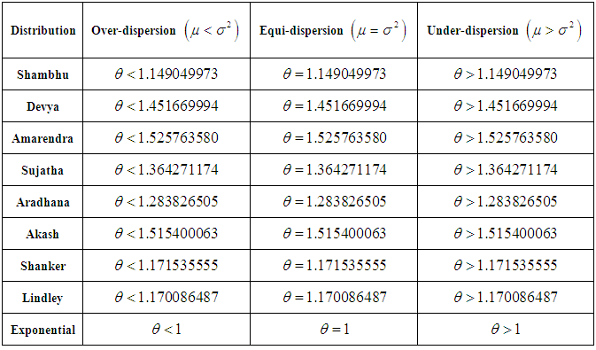
4. Reliability Properties

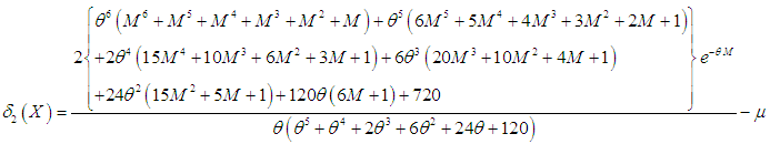
In this section, the important reliability properties of Shambhu distribution including reliability function, , the hazard rate function (also known as the failure rate function), and the mean residual life function, have been discussed. The , and of a continuous random variable having p.d.f., and c.d.f., are respectively defined as

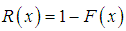(4.1)

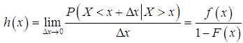(4.2)

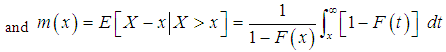(4.3)

The corresponding reliability function, , hazard rate function, and the mean residual life function, of Shambhu distribution (2.1) are thus obtained as

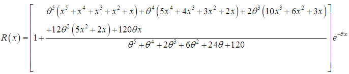(4.4)

(4.5)

and

(4.6)

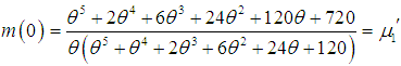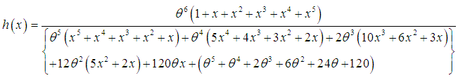
It can be easily verified that and . The graphs of and of Shambhu distribution (2.1) for different values of its parameter are shown in figures 2(a) and 2(b), respectively.

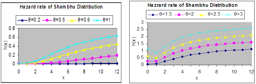Figure 2(a). Graphs of h (x) of Shambhu distribution for selected value of parameter θ

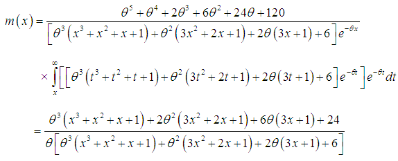
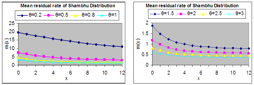Figure 2(b). Graphs of m(x) of Shambhu distribution for selected value of parameter θ

It is also obvious from the graphs of and that is decreasing function for and for and an increasing function of other values of and , whereas is monotonically decreasing function of and .

5. Stochastic Orderings

Stochastic ordering of positive continuous random variables is an important tool for judging the comparative behaviour of continuous distributions. A random variable is said to be smaller than a random variable in the

(i) stochastic order if for all

(ii) hazard rate order if for all

(iii) mean residual life order if for all

(iv) likelihood ratio order if decreases in.

The following results due to Shaked and Shanthikumar (1994) are well known for establishing stochastic ordering of continuous distributions

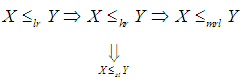The Shambhu distribution is ordered with respect to the strongest ‘likelihood ratio’ ordering as shown in the following theorem:

Theorem: Let Shambhu distributon and Shambhu distribution . If , then and hence , and .

Proof: We have

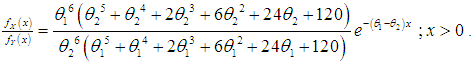Now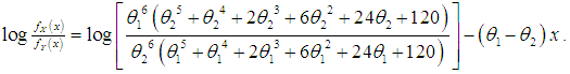

This gives .

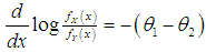Thus for 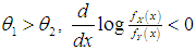. This means that and hence , and.

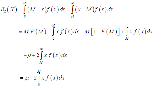
6. Mean Deviations

The amount of scatter in a population is evidently measured to some extent by the totality of deviations from the mean and the median known as the mean deviation about the mean and the mean deviation about the median and are defined as

and , respectively,

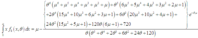
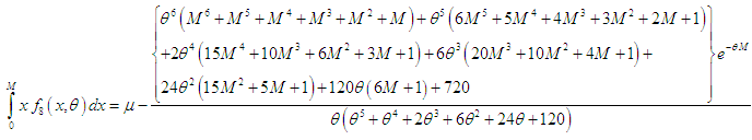
where and .

The expressions for and can be easily calculated using the following simplified relationships

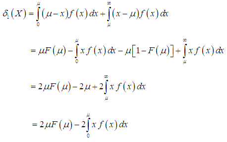(6.1)

and

(6.2)

Using p.d.f. (2.1) and the mean of Shambhu distribution (2.1), we get

(6.3)

(6.4)

Using expressions (6.1), (6.2), (6.3), and (6.4), the expressions for and of Shambhu distribution (2.1), after some algebraic simplification, are obtained as

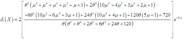(6.5)

and

(6.6)

7. Bonferroni and Lorenz Curves

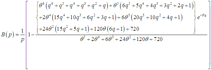
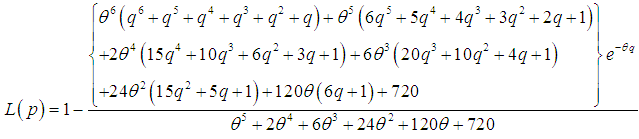
The Bonferroni and Lorenz curves (Bonferroni, 1930) and Bonferroni and Gini indices have applications not only in economics to study income and poverty, but also in other fields like reliability, demography, insurance and medicine. The Bonferroni and Lorenz curves are defined as

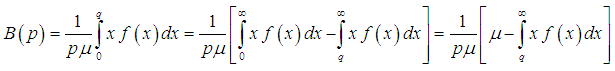(7.1)

and

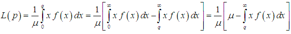(7.2)

respectively or equivalently

(7.3)

and

(7.4)

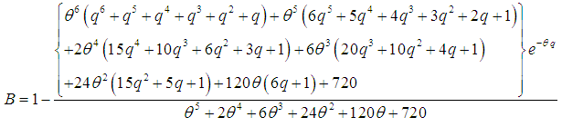
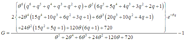
respectively, where and .

The Bonferroni and Gini indices are thus defined as

(7.5)

and

(7.6)

respectively.

Using p.d.f. of Shambhu distribution (2.1), we get

(7.7)

Now using equation (7.7) in (7.1) and (7.2), we get

(7.8)

and

(7.9)

Now using equations (7.8) and (7.9) in (7.5) and (7.6), the Bonferroni and Gini indices of Shambhu distribution (2.1) are obtained as

(7.10)

(7.11)

8. Parameter Estimation

8.1. Maximum Likelihood Estimate (MLE) of the Parameter

Let 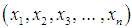be a random sample from Shambhu distribution (2.1). The likelihood function, of Shambhu distribution is given by

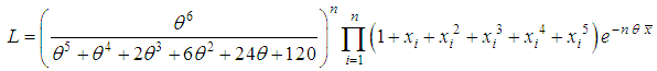The natural log likelihood function is thus obtained as

where is the sample mean.

Now

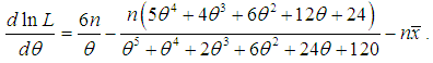The maximum likelihood estimate, of is the solution of the equation and is given by the solution of the following sixth degree polynomial equation in

(8.1.1)

8.2. Method of moment Estimate (MOME) of the Parameter

Equating the population mean to the corresponding sample mean , the method of moment estimate (MOME) , of of Shambhu distribution is found as the solution of the same six degree polynomial equation (8.1.1), confirming that the MLE and MOME of for Shambhu distribution are identical.

9. Illustrative Examples

In this section two examples of real lifetime data-sets have been considered for illustrating the applications and goodness of fit of Shambhu distribution. The following two real lifetime data-sets from medical science and engineering have been used to fit Shambhu distribution using maximum likelihood estimate and the fitting of the distribution has been compared with one parameter lifetime distributions namely exponential, Lindley, shanker, Akash, Aradhana, Sujatha, Amarendra and Devya distributions and the fit has been found to be quite satisfactory.

Data set 1: The first data set represents the lifetime’s data relating to relief times (in minutes) of 20 patients receiving an analgesic and reported by Gross and Clark (1975, P. 105). The data are as follows:

Data set 2: The second data set is the strength data of glass of the aircraft window reported by Fuller et al (1994):

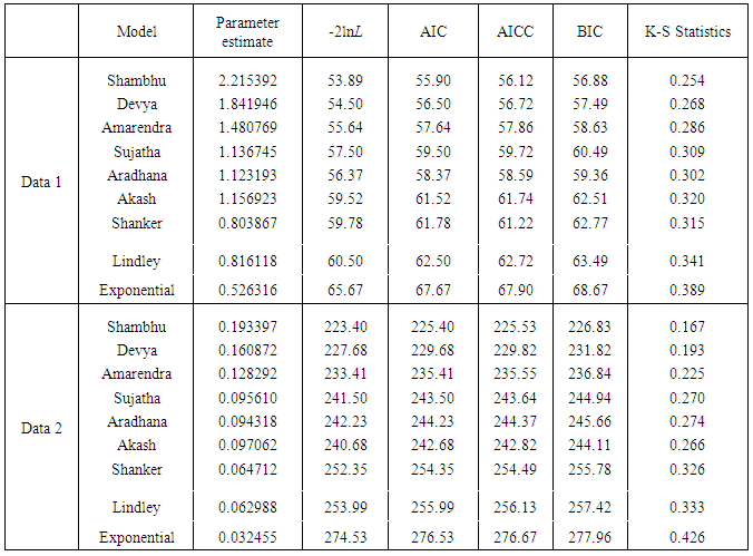
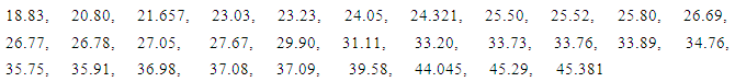In order to compare the goodness of fit of these lifetime distributions, -2lnL, AIC (Akaike Information Criterion), AICC (Akaike Information Criterion Corrected), BIC (Bayesian Information Criterion), and K-S Statistics ( Kolmogorov-Smirnov Statistics) for two real data - sets have been computed and presented in table 2. The formulae for computing AIC, AICC, BIC, and K-S Statistics are as follows:

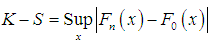, where k = the number of parameters, n = the sample size and is the empirical distribution function.

The best lifetime distribution is the distribution having lowest values of -2lnL, AIC, AICC, BIC, and K-S statistics.

Table 2. MLE’s, -2lnL, AIC, AICC, BIC, and K-S Statistics of the fitted distributions of data sets 1 and 2

It is obvious from the above table that Shambhu distribution gives better fit than exponential, Lindley, Shanker, Akash, Aradhana, Sujatha, Amarendra and Devya distributions and hence it may be preferred over exponential, Lindley, Shanker, Akash, Aradhana, Sujatha, Amarendra and Devya distributions for modeling various lifetime data from biomedical science and engineering.

10. Conclusions

A new lifetime distribution named, ‘Shambhu distribution’ has been proposed to model real lifetime data-sets from medical science and engineering. Its important statistical properties including moment generating function, moments about origin and moments about mean and expressions for skewness and kurtosis, index of dispersion have been obtained. Other interesting reliability properties of the proposed distribution such as reliability function, hazard rate function, mean residual life function have been derived and discussed. The stochastic ordering, mean deviations, Bonferroni and Lorenz curves have also been discussed. The estimation of its parameter has been discussed using maximum likelihood estimation and the method of moments. Two examples of real lifetime data- sets have been presented to show the applications of Shambhu distribution and the goodness of fit of the distribution has been compared to one parameter exponential, Lindley, Shanker, Akash, Aradhana, Sujatha, Amarendra, and Devya distributions.

The future works to be done on Shambhu distribution are to study its size-biased form, truncated forms, weighted forms, and mixture with other discrete distributions.

NOTE: The paper is dedicated in respect of my eldest brother and mentor Professor Shambhu Sharma, Department of Mathematics, Dayalbagh Educational Institute, Dayalbagh, Agra, India.

ACKNOWLEDGEMENTS

The author would like to thank the Editor-In-Chief and the referee for their comments which improved the quality of the paper.