-
Paper Information
- Paper Submission
-
Journal Information
- About This Journal
- Editorial Board
- Current Issue
- Archive
- Author Guidelines
- Contact Us
International Journal of Probability and Statistics
p-ISSN: 2168-4871 e-ISSN: 2168-4863
2016; 5(2): 33-47
doi:10.5923/j.ijps.20160502.02

Time Series Analysis of Interest Rate in Nigeria: A Comparison of Arima and State Space Models
 Abstract
 Reference
 Full-Text PDF
 Full-text HTML
Omekara C. O. , Okereke O. E. , Ehighibe S. E.
Department of Statistics, Michael Okpara University of Agriculture Umudike, Nigeria
Correspondence to: Omekara C. O. , Department of Statistics, Michael Okpara University of Agriculture Umudike, Nigeria.
| Email: |  |
Copyright © 2016 Scientific & Academic Publishing. All Rights Reserved.
This work is licensed under the Creative Commons Attribution International License (CC BY).
http://creativecommons.org/licenses/by/4.0/

This paper set out to analyse and forecast the monthly commercial banks interest rate data on time deposits in Nigeria for a period of 2005-2015. The main objective of this study is to propose an appropriate time series forecasting model for the interest rate data. The data which was obtained from the Central Bank of Nigeria (CBN) was analysed using Autoregressive Integrated Moving Average (ARIMA) procedure, Intervention Autoregressive Integrated Moving Average (Intervention ARIMA) procedure and State Space Modelling approach. As an illustration, the three approaches were compared for modelling and forecasting the interest rate data. Evidence showed Intervention ARIMA model to be more adequate than ARIMA (without intervention) model and State Space Model to be also more adequate than Intervention ARIMA model for the data set (interest rate in Nigeria) under consideration.
Keywords: Interest rate, Forecasting, ARIMA, State Space
Cite this paper: Omekara C. O. , Okereke O. E. , Ehighibe S. E. , Time Series Analysis of Interest Rate in Nigeria: A Comparison of Arima and State Space Models, International Journal of Probability and Statistics , Vol. 5 No. 2, 2016, pp. 33-47. doi: 10.5923/j.ijps.20160502.02.
Article Outline
1. Introduction
- In the recently years, more attention has been drawn to analyzing and forecasting Interest rates. This is particularly because interest rate is a key financial variable that affects decisions of consumers, businesses, financial institutions, professional investors and policymakers. Changes in interest rates have important implications for the economy’s business cycle and are crucial to understanding financial development and changes in economic policy of Nigeria. Interest rates have fundamental implications for the economy, by either impacting on the cost of capital or influencing the availability of credit, by increasing savings, it is known to determine the level of investment in an economy. The importance of interest rate depends on its equilibrating influence on supply and demand in the financial sector [6] and [25]. Interest rates affect consumer spending. The higher the rate, the higher their loans will cost them, and the less they will be able to buy on credit. Interest rates are used by central banks as a means to control inflation. Movements in rates of interest either due to change in money supply or change in demand for money will affect the determination of national and financial institutional (Banks) income.Time-series analysis and forecasts of interest rates can therefore provide valuable information to financial market participants and policymakers.Forecasts of interest rates can also help to reduce interest rate risk faced by individuals and firms. Analysis and forecast of interest rates is very useful to central bank of Nigeria (CBN) in assessing the overall impact of its policy changes and taking appropriate corrective action, if necessary. To achieve the desired level of interest rate, the Central Bank of Nigeria (CBN) adopts various monetary policy tools, key among which is the Monetary Policy Rate (MPR). This rate is the rate at which the Central Bank Nigeria (CBN) is willing to rediscount first class bills of exchange before maturity [26]. He further opined that by changing this rate the CBN is able to influence market cost of funds. If the CBN increases MPR, banks’ lending rates are expected to increase with it, showing a positive relationship. Historically, the interest rate regime in Nigeria has been very stochastic as it varies from month to month and year to year. The central bank of Nigeria kept its benchmark interest rate at 11 percent on January 26th, 2016 as widely expected following an unexpected cut by 200bps at its November 2015 meeting in order to boost growth. The bank also held the cash reserve ratio for commercial banks at 20 percent. Interest Rates in Nigeria averaged 10.03 percent from 2007 until 2016, reaching an all-time high of 13 percent in November of 2014 and a record low of 6 percent in July of 2009. Interest Rates in Nigeria is reported by the Central Bank of Nigeria.Several researchers have worked on interest rates data. [1], examined the implications of interest rate for savings and investment in Nigeria using Pearson’s correlation coefficient and regression analysis. Evidence from their work showed that interest rate was a poor determinant of savings and investment, indicating that bank loans were mostly not used for productive purposes. [22], studied the relationship between interest rate and economic growth in Nigeria. The study employed cointegration and error correction modeling techniques and revealed that interest rate has significant effect on economic growth. [20], on his own studied Interest Rate Targeting: A Monetary Tool for Economic Growth inNigeria? Stakeholders’Approach. The study showed that there was a significant interest rate impact on economy growth in Nigeria. [23], also observed that interest rate can have a substantial influence on the rate and pattern of economic growth by influencing the volume and disposition of savings as well as the volume and productivity of investment. [27], forecasted short-term interest rates using univeriate models: Random walk, ARIMA, ARMA-GARCH and ARIMA-EGARCH and the results show that the interest time series have volatility clustering effect and hence GARCH based models are more appropriate to forecast than the other models. [31], investigated whether there was a linkage of interest rates between the united states, West Germany, and Switzerland during the period of flexible exchange rate, (1974-1984). It was shown that there was strong linkage exist during the second period, but during the first period there was no or only a weekly pronounced linkage.Since authors have used many models and methods of analysing time series data (interest rates) such as ARIMA, ARIMA-GARCH, ARIMA-EGARCH, I(d) statistical models amongst others, the main objective of this study is to propose an appropriate time series forecasting model for the monthly interest rate data in Nigeria using ARIMA, ARIMA Intervention and State Space Models respectively. For this purpose, the study will help to fill the research gap as many researchers seem to have not researched on commercial banks interest rate in Nigeria using ARIMA and State Space models. It will expose researchers and other users of the work to an important field of time series that does not require stationarity (differencing) of time series data before analysis (State Space Modelling technique). This study will confirm if State Space Modelling is more adequate than Box and Jenkins ARIMA Modelling as argued by [12]. This study will also expose the current trend/pattern and level of commercial banks interest rate in Nigeria to researchers, investors, government and users of the work. Finally, it will make recommendations that could enable the government to make and implement policies and programs that will always favour the economic situation of Nigeria at any given time.
2. Research Methodology
- This paper focuses on the analysis of monthly commercial banks interest rate on time deposits in Nigeria for a period of 2005-2015. The data analysed in this paper were obtained from Central Bank of Nigeria statistical bulletin of 2015. The major statistical tools used in this study is time series analysis using Autoregressive Integrated Moving Average (ARIMA), Intervention Autoregressive Integrated Moving Average (Intervention ARIMA) and State Space Modelling approaches.
2.1. Box-Jenkins (ARIMA) Process
- The general ARIMA (p,d,q) process can be written in the general form:
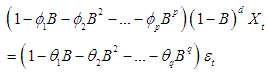 | (2.1) |
2.2. Intervention ARIMA Model
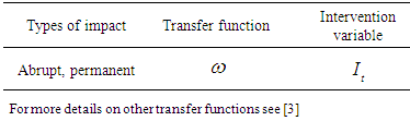
- This is a special kind of ARIMA model with input series. It is also called an interrupted time series model. In an intervention model, the input series is an indicator variable that contains discrete values that flag the occurrence of an event affecting the response series. This event is an intervention in or an interruption of the normal evolution of the response time series, which, in the absence of the intervention, is usually assumed to be a pure ARIMA process. Intervention models can be used both to model and forecast the response series and also to analyze the impact of the intervention. Intervention analysis, introduced by [3] provides a framework for assessing the effect of an intervention on a time series under study. Given the model
 where
where  is the change in the mean, and
  is modeled as some ARIMA model where there is no intervention. The Time Series
  is called the pre-intervention data.
|
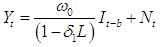 | (2.2) |
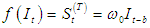 . Also, if there is no time delays (b=0), then
 and the full model will now be of the form;
  | (2.3) |
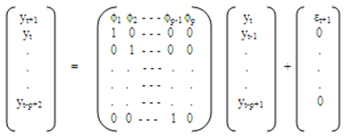
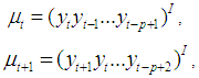
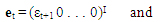
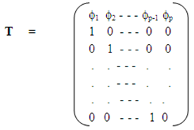
2.3. State Space Modelling Approach
- [12] argue that the Box-Jenkins approach is fundamentally problematic since real series are never stationary especially in economic and social fields, however much differencing is done to make it stationary. The authors argue that rather than using Box-Jenkins (ARIMA), it is better to use state space methods, as stationarity of the series is not required. State space model (SSM) refers to a class of probabilistic graphical model that describes the probabilistic dependence between the latent state variable and the observed measurement [14]. The state or the measurement can be either continuous or discrete. The most well studied SSM is the Kalman filter, which defines an optimal algorithm for inferring linear Gaussian systems. The main purpose of SSM time series analysis is to infer the relevant properties of unobserved series of vectors µt’s from a knowledge of the observations yt’s. Other purposes include estimation of parameters and forecasting. The simplest model for a univariate time series (Yt : t = 1, 2, . . .) is the so-called random walk plus noise model (or local level model), defined by
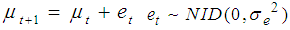 | (2.4) |
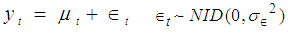 | (2.5) |
 | (2.6) |
 | (2.7) |
 | (2.8) |
 | (2.9) |
 | (2.10) |
 | (2.11) |
 satisfying (2.11) lies inside the unit circle [28].
2.4. Model Selection Criterion
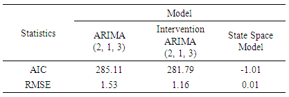
- The estimated models are compared based on the predictive power using the three forecasting accuracy measures: Akaike information criterion (AIC), Root mean square error (RMSE) and Visual comparison of 2015 forecasted values.
 | (2.12) |
 | (2.13) |
3. Results and Discussions
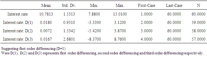
- Figure 1 is the time plot of the monthly interest rate data for the period of 2005-2015.
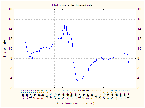 | Figure 1. Time Plot of the Original interest rate data (2005-2015) |
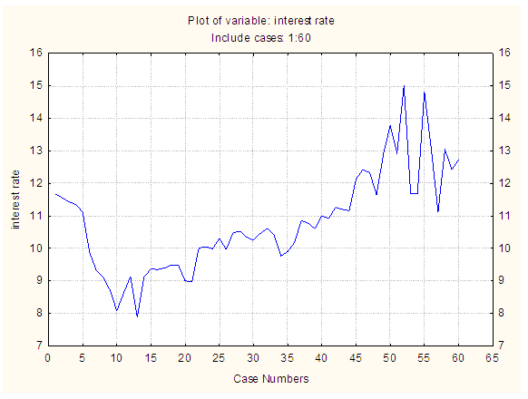 | Figure 2. Time Plot of the Pre-Intervention series of the interest rate (1-60 data points) |
|
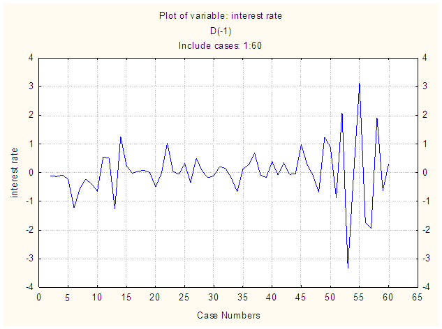 | Figure 3. Plot of the first difference of the pre-intervention series |
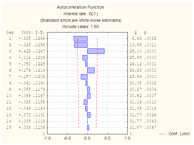 | Figure 4. ACF plot of the first difference of the pre-intervention series |
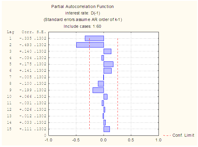 | Figure 5. PACF plot of the first difference of the pre-intervention series |
 | Figure 6. ACF plot of the pre-intervention residual series |
 | Figure 7. PACF Plot of the pre-intervention residual series |
|
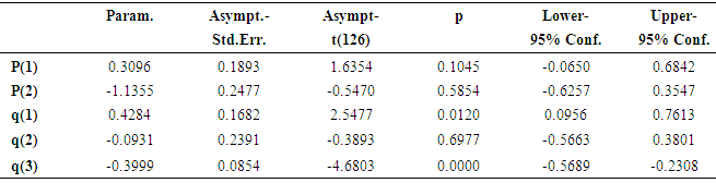
 | (3.1) |
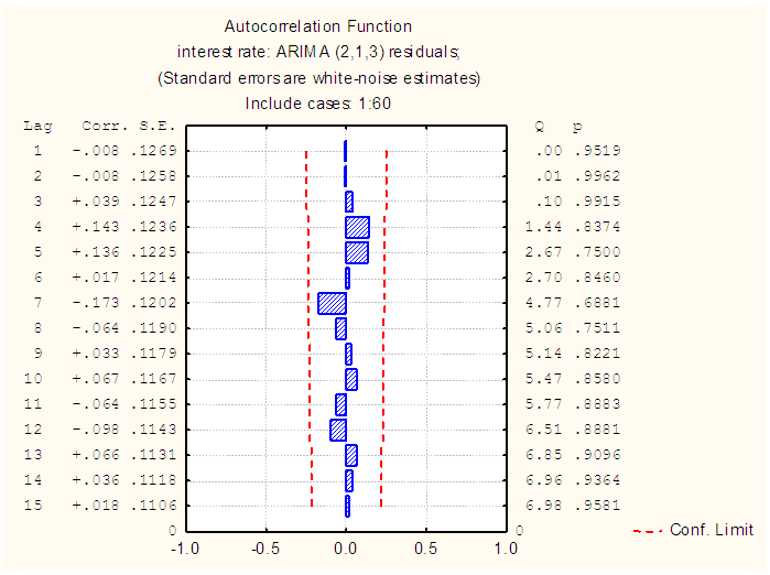
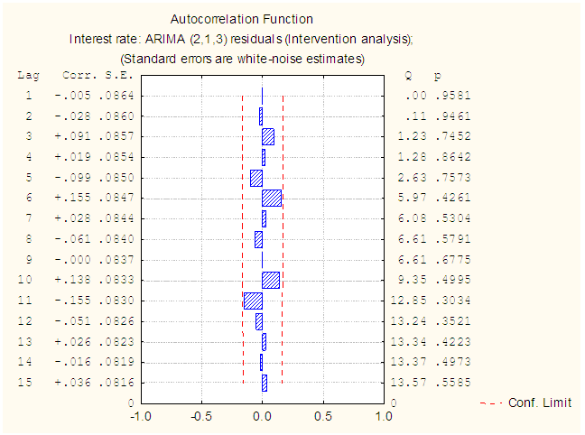 | Figure 8. ACF Plot of the intervention residual |
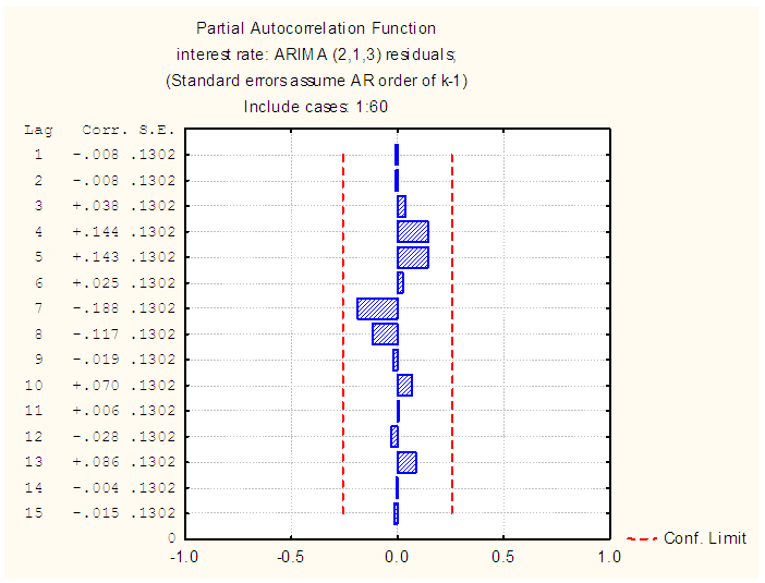
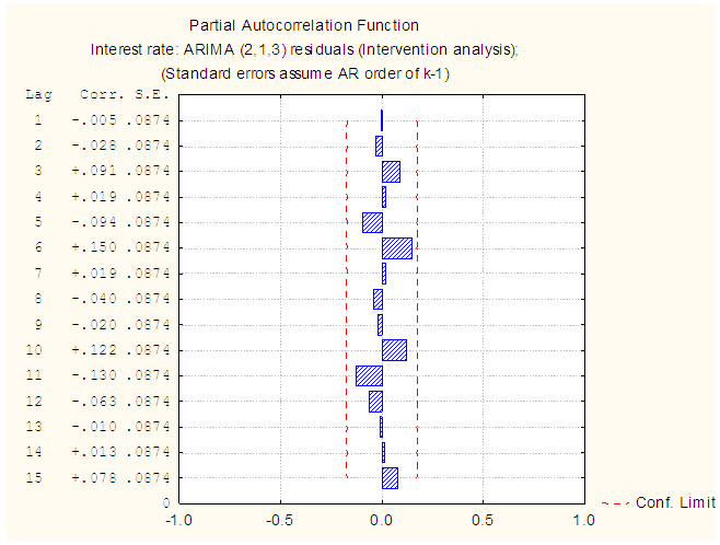 | Figure 9. PACF Plot of the intervention residual |
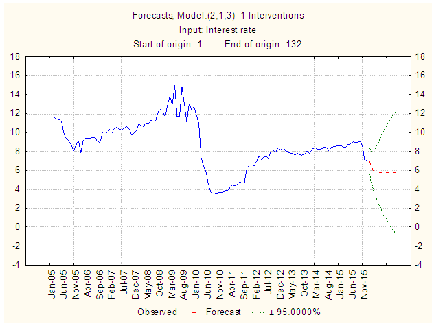 | Figure 10. Time Plot of the interest rate series (2005-2015) and its forecast (2016) |
|
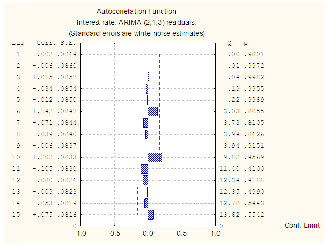 | Figure 11. ACF Plot of the residual (without intervention) |
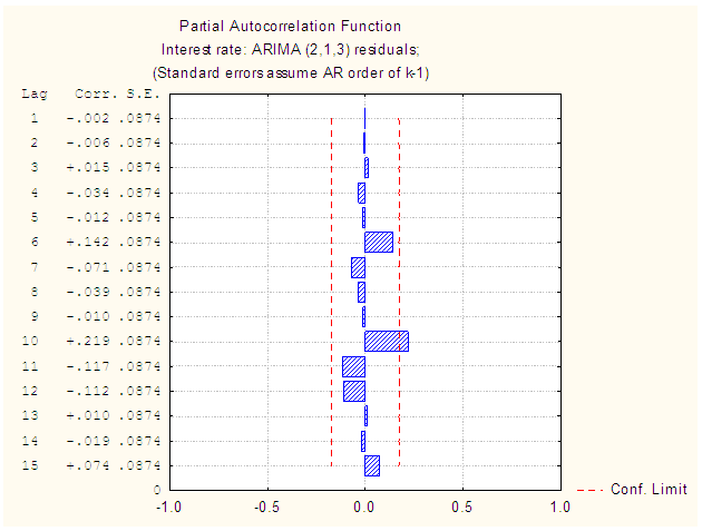 | Figure 12. PACF Plot of the residual (without intervention) |
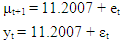 | (3.2) |
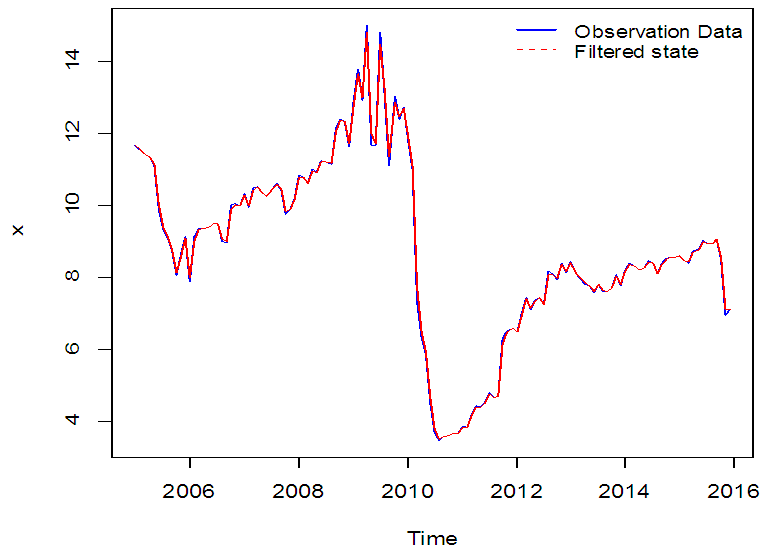 | Figure 13. Plot of the Observed Data and Filtered State |
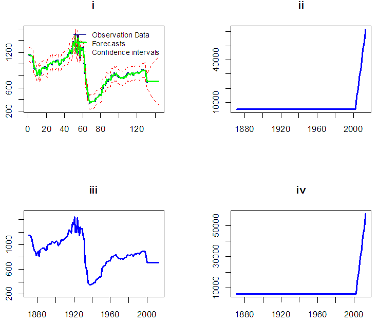 | Figure 14. Plots of filtered States, its variance and Observation series, its variance |
|
4. Summary/Conclusions
- Time series analysis of interest rate data (of Commercial Banks on Time Deposits in Nigeria) from the period of (2005-2015) was carried out in this study. A sudden downward jump in the series after point 60 (January 2010) was observed. This suspected to have been cursed by the Central Bank of Nigeria through their former governor Lamido Sanusi who said in January, 2010 that Nigeria will keep interest rate low so as to boost the economy even as the inflation outlook becomes more uncertain because of rising government spending. Intervention ARIMA (2, 1, 3) and ARIMA (2, 1, 3) models were estimated with the aid of STATISTICA software and it was confirmed that the intervention has an abrupt, permanent change to the interest rate data. State Space (local level) model was also estimated with the aid of R software. Comparison between the estimated ARIMA (2, 1, 3), intervention ARIMA (2, 1, 3) and state space models were made and the result confirmed state space model to be more adequate. Thus, for the data set (interest rate in Nigeria) under consideration, State Space Modelling technique performs better than the ARIMA approaches.
5. Recommendations
- The researchers therefore recommend that the interest rate trend should often be properly monitored to know its level at any given time since it is a nebulous concept. Researchers should always go into modelling of interest rate data so as to monitor and control the effects that sudden changes in interest rate could cost to our economy. We also encourage researchers to go into State Space Modelling technique as it has been confirmed more adequate than ARIMA techniques in analysing especially time-series data (interest rate in Nigeria). Finally, we recommend that government (through CBN) should always amend our monetary policies or implement new ones that will always monitor the level of interest rate in Nigeria and set it in the way it will always favour the current economic situation of Nigeria at any given time.